


In many of the problems dealt with in this book, the
number of trials, n, is very large. A small molecule
undergoing diffusion, for example, steps to the right or left
millions of times in a microsecond, not 4 times in a few
seconds, as the ball in the apparatus of
Fig. A.3. There are
two asymptotic limits of the binomial distribution. One,
the Gaussian, or normal, distribution, is obtained when
the probability of a success, p, is finite, i.e., if np ->
 as
n -> . The other, the
Poisson distribution, is obtained if
p is very small, so small that np remains finite as
n -> .
as
n -> . The other, the
Poisson distribution, is obtained if
p is very small, so small that np remains finite as
n -> .
The derivation of the Gaussian distribution involves the use of Stirling's approximation for the factorials of the binomial coefficients:
where e is the base of the natural logarithms. The result is
where µ = <k> = np and
If we define u = (k - µ) /
P(u) is called the normal curve of error; it is shown in
Fig. A.5. As an exercise, use your tables of definite
integrals and show that
and
Eq. A.30 can be done by inspection: P(u) is an even
function of u, so uP(u) must be an odd function of u. The
distribution P(u) is normalized, its mean value is 0, and its
variance and standard deviation are 1.
Figure A.5. The normal curve of error: the
Gaussian distribution plotted in units of the standard deviation
 = (<k2> -
<k>2)1/2
= (npq)1/2, as before. P(k; µ,
) dk is the probability
that k
will be found between k and k + dk, where dk is
infinitesimal. The distribution is continuous rather than discrete.
Expectation values are found by taking integrals rather
than sums. The distribution is symmetric about the mean,
µ, and its width is determined by
. The area of the
distribution is 1, so its height is inversely proportional to
.
, i.e., plot the distribution
with the abscissa in units of
and the origin at
µ, then
= (<k2> -
<k>2)1/2
= (npq)1/2, as before. P(k; µ,
) dk is the probability
that k
will be found between k and k + dk, where dk is
infinitesimal. The distribution is continuous rather than discrete.
Expectation values are found by taking integrals rather
than sums. The distribution is symmetric about the mean,
µ, and its width is determined by
. The area of the
distribution is 1, so its height is inversely proportional to
.
, i.e., plot the distribution
with the abscissa in units of
and the origin at
µ, then
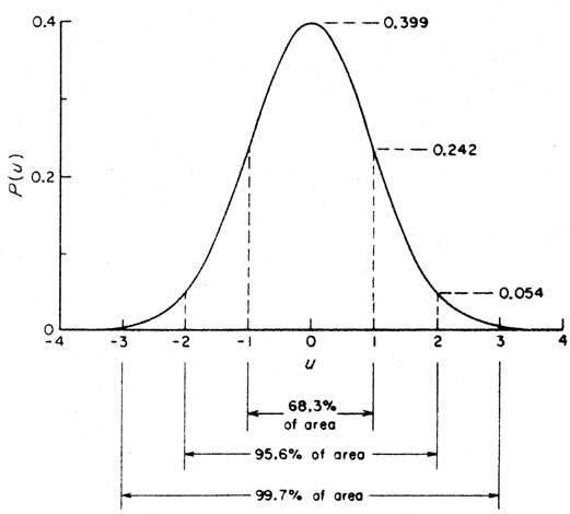
with its origin at the mean
value µ. The area under the curve is 1. Half the area falls
between u = ± 0.67.