


2.3.5. Extragalactic Distance Indicators
To reach to distances beyond 4 Mpc, a variety of extragalactic distance indicators have come into existence. Most of these indicators are calibrated against the distance to the LMC, M31 and M33. The five most reliable and well-used extragalactic distance indicators are the following:
The Tully-Fisher relation
This was originally used by Opik in 1922 and is basically a dynamical method for determining intrinsic luminosity. The argument works as follows:
Circular velocities in galaxies scale as:

| (8) |
Using the Mass-to-Light (M/L) ratio, mass can be parameterized as
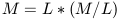
| (9) |
If we assume that disk galaxy surface brightness (SB = galaxy luminosity per unit area) is same for all spirals then we can write L in terms of R and SB as follows:

| (10) |
So now equation 10 becomes:
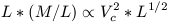
| (11) |
If we now further assume that M/L is constant we then have the simple expression:
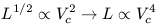
| (12) |
Converting to magnitude units and remembering that M = -2.5 log L, we arrive at the predicted slope in the relation involving M and Vc
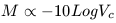
| (13) |
The methodology used to derive equation 13 has the implicit assumption that the luminous matter dominates the mass of galaxies and the effects of dark matter on the gravitational potential and hence Vc are explicitly not considered, even though it is likely that the masses of galaxies are dominated by dark matter (see Chapter 4). It is thus quite paradoxical that equation 13 has been empirically verified numerous times. This verification indicates that rotating disk galaxies scale their rotation velocities by their luminosities despite being dark matter dominated. Hence, there must be some fine-tuned coupling between the amounts of dark and light matter in galaxies that we simply do not understand. Because of this possible fine-tuning, it is difficult to argue that the Tully-Fisher (TF) relation has a real basis in physics. Rather, its an empirical relation that seems to work remarkably well.
For the TF relation to work, 3 things must be adhered to by all rotating disk galaxies and each of these 3 things represents a potential failure point (or at least a point of systematic error) in the derivation of extragalactic distances.
1. Galaxies must be circularly symmetric in order to properly correct the observed circular to the plane of the galaxy to derive Vc. To first order they are. To second order, galaxies could be embedded in dark matter halos which are flattened and this would cause systematic deviations from circular motion which would produce dispersion in the TF relation. A systematic dependence of halo flattening on galaxy environment would produce systematic zero point shifts in the TF relation (see de Zeeuw and Franx 1992, Rix and Zaritsky 1995).
2. Galaxies must have the same M/L ratio. In reality, this is absurd as clearly, the stellar population differences in galaxies produce differences in M/L. However, if the stellar mass is a very small percentage of the total mass, then M/L variations associated with stellar population differences are relatively minor. Still, for the TF relation to work at all, these dark matter dominated galaxies must somehow be programmed to produce a certain amount of luminous matter so that galaxy obeys the TF relation! This brings up the serious possibility that small but systematic differences in dark matter content produce systematically different zero points in the TF relation. The lack of any identified third parameter in the TF relation, despite a wealth of observational attempts to find one, argues that these systematic effects are subtle (e.g., Bernstein et al. 1994; Feast 1994; Persic and Salucci 1991; Biviano et al. 1990; Mould et al. 1989; Giraud 1987)
3. Galaxies must have the same surface brightness. This is clearly even more absurd than the M / L requirement. In fact, an entire chapter in this book is devoted to the subject of Low Surface Brightness (LSB) galaxies whose very existence straightforwardly shows that disk galaxy SB can not be constant. Interestingly, LSB galaxies do define a TF relation like that of normal galaxies, although the scatter is much larger (Sprayberry et al. 1995). Moreover, surface brightness issues are only important if the calibration sample has a different range in surface brightness (over the same range in Vc) as the distant sample; only then will a systematic offset occur (see Bothun and Mould 1987). This is relevant to the case of M33 as a fundamental calibrator of the TF relation in that it is generally of higher SB than other galaxies of similar Vc.
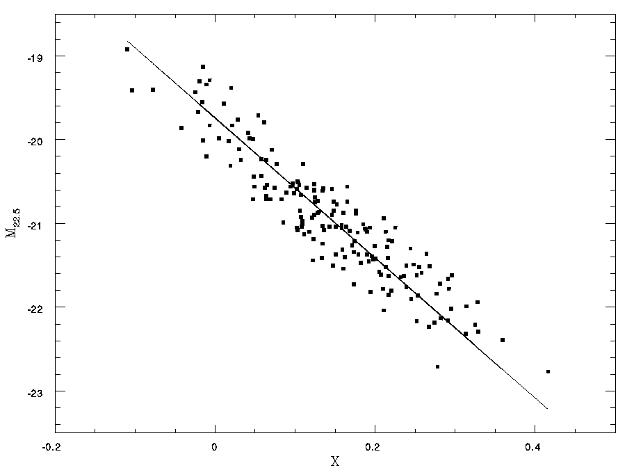
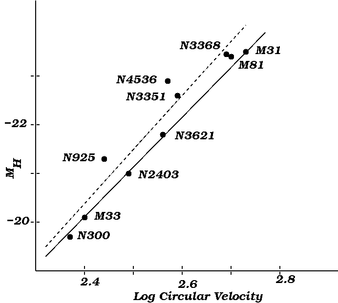
Despite the fact that galaxies do not all have the same SB or M/L there remains a good correlation between Vc and luminosity in almost any sample of inclined disk galaxies. Figure 2-9 shows a recent example of this good correlation where the data come from Dell'Antonio et al. (1996). While much of scatter around this relation is due to measurement errors, some of the scatter is intrinsic. Unfortunately, the intrinsic scatter of the TF relation is not well known and estimates range from 0.1 - 0.7 mag. In principle, if this intrinsic scatter is low then calibration of the TF relation requires only two points. This requirement can be meet by M33 and M31. It is desirable, of course, to increase the calibration sample in case the intrinsic scatter is moderately large. Some investigators choose to increase the calibration sample by including Local Group galaxies which are less massive than M33. It is our opinion that this is not good practice since the circular symmetry of low mass galaxies is seriously in question. Ideally, one wishes to add spiral galaxies with Vc between that of M33 and M31. There are 5 such nearby spiral galaxies now available (Images of each galaxy are available at the Web site). Each of these galaxies is in the HST Key project program to determine Cepheid distances.
|
Figure 2-9: Example relation between rotational velocity and I-band luminosity for a large sample of spiral galaxies from Dell'Antonio et al. (1996). The slope of the line is -8.4, which is close to the expected slope -10 relation derived from the Virial Theorem. The X-axis is the log of the line width where zero corresponds to log = 2.5 (~ 300 km/s). |
 M81: The best determination
of its distance comes
from Freedman et al. (1994) using Wide Field Planetary Camera (WFPC)
data from HST to identify and
measure Cepheid variables. This distance
is (m - M) = 27.80 ± 0.20 (which assumes an LMC modulus
of 18.5).
M81: The best determination
of its distance comes
from Freedman et al. (1994) using Wide Field Planetary Camera (WFPC)
data from HST to identify and
measure Cepheid variables. This distance
is (m - M) = 27.80 ± 0.20 (which assumes an LMC modulus
of 18.5).
NGC 2403: This galaxy has a
slightly higher Vc
than M33 but overall is very much like M33. HST observations of
NGC 2403 have not yet been concluded at the time of this
writing. Ground-based measurements of its
Cepheids yield a distance modulus of 27.46 ± 0.24.
NGC 300: This is a very low
mass, but rather high
SB spiral galaxy. It has Vc less than M33 and
its not clear if it should be used as a TF calibrator.
A Cepheid distance of (m - M) = 26.0 ± 0.2 has been derived
from observations of a few Cepheids.
NGC 925: This is a late type
spiral galaxy which is
somewhat barred and shows multiple spiral structure like NGC 2403.
It is a member of the NGC 1023 group of galaxies which also
contains NGCs 891, 949, 1003, 1023 and 1058. All of these galaxies
have had recent determinations of their distance (see
Ciardullo et al. 1991, Pierce 1994, Tonry 1993, or Schmidt et al.
1992). The mean distance modulus to the NGC 1023 group that results is
(m - M) = 29.98 ± 0.12 (mean error). Using an LMC distance
modulus of 18.5 Silbermann et al. (1996) derive (m - M) = 29.84 ± 0.16
from WFPC observations of its Cepheids. Interestingly,
Silbermann et al. (1996) derive a moderate level of mean reddening
for these Cepheid which again underscores the need to estimate individual
reddenings from multicolor photometry.
NGC 3351: This is a barred
spiral which is a member of the
Leo I Group of galaxies. Leo I is an important group because it contains
the two nearest bright elliptical galaxies (NGCs 3377 and 3379). As
will be clear later, its important to have a collection of spirals and
ellipticals in the same group to check for the consistency of different
kinds of distance estimators as applied to different kinds of galaxies.
HST observations of its Cepheids by Graham et al. (1996) yield a distance
modulus of (m - M) = 30.01 ± 0.19.
In principal, these 5 spiral galaxies, in addition to M31 and M33 provide a better calibration of the TF relation. This new calibration is shown in Figure 2-10 where it can be seen that NGC 925 and NGC 3351 lie significantly off the relation defined by just M31 and M33. Thus, the addition of more calibrating galaxies, while in principal is a good idea, in practice is likely revealing the intrinsic scatter and subtle galaxy-galaxy differences in the TF relation.
|
Figure 2-10: Available sample of Local galaxies for the calibration of the Tully-Fisher relation. Most of these galaxies have had new distance determinations from the Hubble Space Telescope Key Project (see Rawson et al. 1997). Solid line represents the relation defined only by M33 and M31; dashed line is the best fit to all the calibrating galaxies. |
The Luminosity Function of Planetary Nebulae
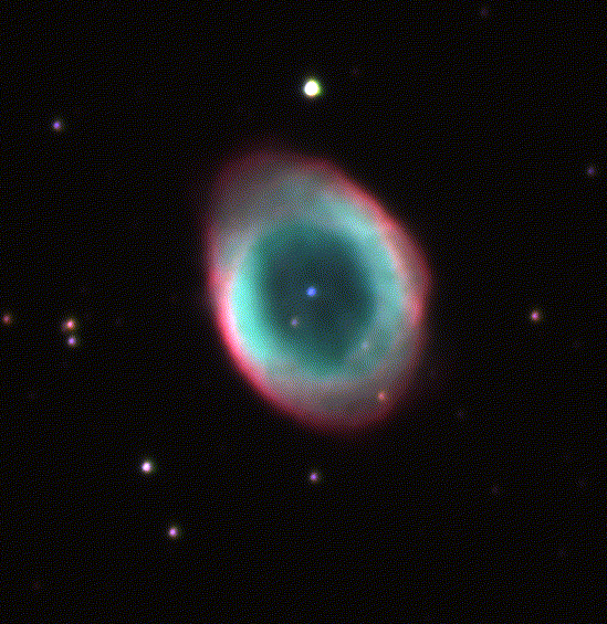
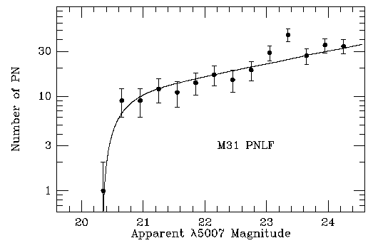
Planetary nebulae are evolved stars that are ejecting their outer envelopes. An example is shown in Figure 2-11. The physics of this phenomenon are universal and the evolutionary rates are so rapid in this phase that virtually all currently detectable planetary nebulae in a given galaxy occupy a very small mass range. As the ionizing flux depends upon this mass, the luminosity of a planetary nebulae, as measured in the [O III] emission line, should be nearly constant from nebulae to nebulae. Slight differences in mass (and perhaps metallicity), which arise from differences in stellar population ages within a galaxy, produces a range in luminosity which hence defines the luminosity function of Planetary Nebulae (PNLF). Figure 2-12 shows the PNLF for M31. There is a very sharp cutoff in the maximum luminosity which can be used as a standard candle for distance estimates. The main limitations of the PNLF method are the following:
It is best applied to
elliptical galaxies which have
less dispersion in the ages of the stellar populations that will
produce the planetary nebulae. Applying it to spiral galaxies
is slightly more problematical as a range of stellar population
ages contributes to the PNLF.
There is no good way to
determine distances to galactic
PN and therefore the PNLF does not have zeropoint which can be based
on any galactic calibration. Currently, it is the distance to M31
that sets the zeropoint for the PNLF.
The method is limited to
distances out to about
the Virgo cluster. Beyond that, PN become pretty faint
for ground-based telescopes.
As in the case of Red
Supergiants, the PNLF may depend
on the total number of stars in the galaxy. Indeed, Bottinelli
et al. (1991) - do find a small dependence of distance modulus on
galaxy luminosity, in the sense that the more luminous galaxies
have smaller distance moduli. Sandage (1994) has taken the
extreme position that this population bias is far more severe
than the proponents of the PNLF method (Jacoby et al. 1992) realize.
Examining the actual data (e.g., Figure 2-12),
however, shows that the PNLF does have
a relatively sharp cutoff at some maximum luminosity but there
is insufficient data to reliably measure the intrinsic scatter
at the bright end of the PNLF. This likely introduces a small
systematic error.
Recent observations of the
UV light of elliptical
galaxies by Brown et al. (1995) indicates that the
UV light is dominated by the kinds of stars (e.g., Post Asymptotic
Branch stars) that are the ionizing
stars in PN. They find small differences in mean mass of these PAGB
stars from one
elliptical to another. These mass differences will cause differences
in the luminosity of the [O III] line in PN and thus will produce
some scatter in the PNLF. The mass differences are generally around
0.01 - 0.03 solar masses and it is unclear how much scatter in the PNLF
is actually introduced by mass differences this small.
|
Figure 2-11: Example Planetary Nebula where the outer atmosphere has been shed and is now ionized by the central star. The mass of the central star determines the ionization rate and the subsequent emission line luminosity of the planetary nebula. This image is a true-color CCD image obtained by Nelson Caldwell of the Smithsonian Astrophysical Observatory. |
|
Figure 2-12: The PNLF for M31 courtesy of Robin Ciardullo. The sharp cutoff in maximum luminosity, if universal, can be used as the reference luminosity for distance determinations to other galaxies. In this case, the distance to M31 serves as the fundamental calibration. |
On the positive side, PNLF distances, calibrated from the PNLF for M31, for 4 galaxies (2 ellipticals and 2 early type spirals) in the Leo I group yield a set of distances that are self-consistent to an accuracy of 5%. Furthermore, these distances agree well with the Cepheid distance scale for NGC 3351 cited earlier.
Surface Brightness/Luminosity Fluctuations
This is a statistical method which is based on the precepts of Baum and Schwartzschild (1958). It is meant to provide information in the stellar population, specifically the giant branch, for a stellar cluster or galaxy which is at known distance. An inversion of this process as applied to the extragalactic distance scale has been championed by John Tonry and collaborators in various publications (see for instance, Tonry et al. 1996). Rather than explain the theory it is best just to give a practical example of how the method is applied:
Suppose we image an elliptical with a detector with scale 1 arc-second = 3 pixels. We determine that the intrinsic r.m.s. pixel-to-pixel fluctuation signal in the galaxy image is 10% (we have already subtracted out the sky fluctuation signal and the intrinsic luminosity gradient within the galaxy). We then assume that the light from the galaxy is dominated by one kind of star. In this example we assume that it is a K0 star, which has an intrinsic MV = +0.7 and B - V = 0.85. We do the observations in the blue. The 10% fluctuation signal comes from the Poisson noise in the distribution of K0 stars per pixel. Thus the fluctuation signal is N1/2 / N. For the case of 0.1, N = 100. The combined luminosity of 100 K0 giants is MV = -3.5. We also measure that the mean surface brightness of the galaxy over which we measure the fluctuations is b = 20.0 mag arc sec-2. At our pixel scale, 1 pixel would then correspond to a magnitude of 22.5 and each pixel has an absolute magnitude of -3.5. The distance modulus to this galaxy is therefore (m - M) = 22.5 -( -3.5) = 26.0.
Tonry et al. (1996) have refined this basic technique using multicolor photometry. They conclude that fluctuation magnitudes in the I-band are the most practical to measure. As this fluctuation signal is dominated by giants, then differences in individual temperatures and luminosities between the giant stars produces a color dependence on the fluctuation magnitude. This is easily understood as cooler giant stars tend to be more luminous. From direct observations as well as theoretical estimates from stellar population models, Tonry et al. (1996) derive a relation between the average absolute fluctuation magnitude and the color of the stellar population:
| (14) |
Distances can be derived by measuring
 and V - I and
correcting for reddening and then using equation 14.
and V - I and
correcting for reddening and then using equation 14.
The limitations in the application of the Surface Brightness Fluctuation (SBF) method to determining extragalactic distances are the following:
The method is really best
applied to single-age
stellar populations such as those that hypothetically exist
in elliptical galaxies or the bulges of spiral galaxies. Furthermore,
it is sensitive to small scale features such as globular clusters
and/or structure in the dust distribution. To first order these
effects can be identified and removed but they may still leave some
residual signal that contributes to the observed value of
.
In reality, it is not one
single kind of star that
dominates the fluctuation signal but rather the entire
stellar luminosity function, which must be estimated by some
a priori criteria or some observational constraints (such
as broad-band colors). In the case of giant dominated luminosity
fluctuations there should be correlated color fluctuations.
In practice, the variation in K/M giant ratio per pixel can be
determined via this correlation. Very good data is required to
see these color fluctuations as the sky fluctuations at
wavelengths greater than 7400 Angstroms become severe. To a large
extent, the recent work that has resulted in equation 14 overcomes
this limitation.
Determining the zeropoint of
the SBF method is extremely
difficult. The only Galaxy in the Local Group that the method
works well for is M32 but it seems unlikely that the giant branch
in M32 is very similar to that in more luminous
ellipticals (see
for instance Silva and Elston 1992). One
can attempt to use the bulge of M31 but there are severe complicating
effects such as small scale dust, possible small-scale stellar clusters,
and cool luminous giants in a metal-rich population, that can all
conspire to give a fluctuation signal unique to M31. It is also
possible to determine the zero point directly from theoretical
considerations (e.g., Worthey 1993). In fact, the zeropoint of this
method used by Tonry (1991) is 0.35 mag brighter than the zeropoint
derived by Tonry et al. (1996). In general, this is a signature of
a still evolving method. The 1991 zeropoint, however, was only based
on M31 and M32 and used a different color-term than the one found
by Tonry et al. (1996) based on a much larger data sample and a better set
of theoretical models.
The Luminosity of Supernovae:
If the maximum luminosity of supernovae of Type Ia or type II is a constant, then they will provide the fundamental determination of the extragalactic distance scale as their high intrinsic luminosity allows detections at very large distances. Indeed, some particularly optimistic groups hope to use this as a means for estimating the deceleration parameter (equation 1.17) of the Universe by measuring the rate of change of H0 over look-back times of a few billion years (see Perlmutter et al. 1995). This is possible because the high intrinsic luminosity of supernovae allow them to be detected at cosmological distances.
Supernova of type II (which come from the detonation of very massive stars) are known to have considerable variation in their luminosity. However, for these supernova one can apply a kinematic model to the expanding photosphere to relate changes in radius to an absolute distance once an accurate radial velocity curve is measured. This method, called the Expanding Photosphere Method (EPM) is similar to the Baade-Wesselink method as it basically compares the angular size of the photosphere with its measured expansion velocity. The method requires a good observational determination of the SN radial velocity curve and a good estimate of the reddening. Application of this method to the type II SN 1987A in the LMC can provide its zeropoint but differences in metallicity and SN environment likely preclude that zeropoint from being universal. Other possible zeropoints include Type II SN that have occurred in M81 and M101. The recent Cepheid distance to M101 based on HST observations by Kelson et al. (1995) gives (m - M) = 29.34 in excellent agreement with the EPM distance of (m - M) = 29.35. The EPM distance to M81, however, is 25% smaller than the HST Cepheid distance found by Freedman et al. (1993).
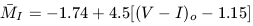
The most recent use of EPM is by Schmidt et al. (1994) for a small sample of Type II SN out to distances of 14,000 km s-1. The method is promising but still prone to large error bars (see data in Figure 2-13) and requires a very good model atmosphere to understand the evolution of effective temperature as that controls the overall spectral shape. In addition, EPM does not yet have a secure zeropoint. Full details of EPM are given in Eastman et al. (1996).
|
Figure 2-13: The EPM distances to 16 Type II supernova vs redshift of the host galaxy, corrected for Virgo Infall. Data are from Schmidt et al. (1994). The solid line shows the best fit for the sample. While there is significant scatter about the relation, the technique does show promise. The initial calibration by Schmidt etal (1994) yields H0 = 73. Notice however, that most of the available sample is local and hence subject to significant peculiar velocities. |
Supernova of type Ia are thermonuclear explosions of degenerate white dwarfs near the Chandrasekhar limit (cf. Wheeler & Harkness 1990), or perhaps mergers of WDs in a binary system (Paczynski 1985). Either detonation or deflagration models (Nomoto et al. 1976; Arnett 1969) then produce the visible energy release that characterize the SNe light and velocity curves. Detailed models show considerable differences in these scenarios (Khokhlov et al. 1993), but their large intrinsic luminosity coupled with the assumed universal physics involved in the Chandrasekhar mass limit have led to strong statements concerning the use of SNe Ia as distance indicators (Branch & Tammann 1992) as they are thought to be standard candles. However, this point remains controversial as there is a demonstrable spread in real, Supernova Ia luminosities (see immediately below).
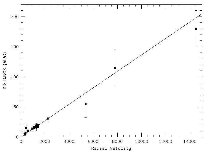
In addition, Phillips (1993) first pointed out a correlation between the supernova luminosity and its decay with time (usually over a 2--3 week period). Hence, one can also use the form of the supernova light curve as a second parameter in estimating supernova luminosity and hence distance. Application of the use of the luminosity-decline rate relation to SN Ia can reduce their luminosity scatter down to ± 0.3 mag making them competitive with other distance indicators (see more below). Particularly optimistic uses of this relation, combined with analysis of multicolor supernova light curve shapes, have yielded an apparent dispersion as low as 0.12 mag (see Reiss et al. 1996). This is shown in Figure 2-14 and it certainly paints an optimistic picture for the use of these objects as distance indicators although von Hippel et al. (1997) show why one should consider this treatment with some skepticism.
|
Figure 2-14: Hubble diagram for Supernova Ia whose distances have been derived using multi-color light profiles and corrections as described in Riess et al. (1996) and whose data is reproduced here. The scatter in this data is 0.12 mags, making it potentially best extragalactic distance indicator available. The initial calibration by Riess et al. (1996) yields Ho = 64. |
The complications to deriving distances from SN luminosity or evolution of its expanding photosphere are the following:
The supernova must be
detected and measured at the time of
maximum light. The rise to maximum can be very sudden (timescales
of hours). Early detection of supernova is therefore critical and this
is extremely difficult to do observationally. Hence, the available sample
of SN II for calibration is necessarily limited.
Reddening estimates towards
supernovae are notoriously difficult
to determine. Spectroscopy of the supernova (SN) itself can give some
constraints if the intrinsic spectrum is understood. Broad-band color
evolution also has constraining power but requires good observations at
the time of maximum light.
The physical mechanisms
which produce supernovae are not well
understood enough to be comfortable with predicting that their maximum
luminosity should be a constant. Indeed, there is now a very good
indication that SN Ia have a significant spread in peak luminosity.
Phillips (1993) has compiled data on 9 SN Ia to galaxies which have
had distances determined via other techniques (e.g. TF relation) and
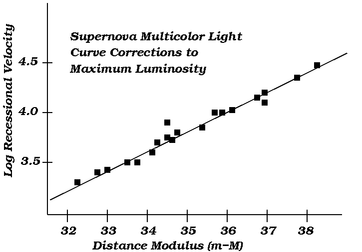
finds a dispersion in peak magnitude of 0.6 mag with a total spread
of 1.6 magnitudes. This spread is also seen in the larger Calan-Tolo
survey as shown in Figure 2.15. However, this
large range or dispersion
in SN Ia luminosity does not preclude their usefulness as a distance
indicator because there is a very tight relation between the maximum
SN Ia luminosity and the rate at which the luminosity declines (see
Hamuy et al. 1995).
|
Figure 2-15: Distribution of intrinsic Supernova Ia luminosities for the Calan-Tololo sample (see Hamuy et al. 1995; von Hippel et al. 1997). To effectively use Supernova Ia luminosity as a distance indicator requires significant compression of this intrinsic luminosity range by using luminosity corrections of the type adovated by Riess et al. (1996) and Hamuy et al. 1995. |
An accurate calibration of
the supernova luminosity scale would
require a supernova occurring in M31 or M33. Eventually one will occur
but astronomers are sufficiently impatient in finding
H0 that secondary
calibrating galaxies, in which a SN Ia did occur, are used. These secondary
galaxies such as NGC 5253, NGC 5128 or IC 4182 have distances of 3-8
Mpc which have been determined mainly from Cepheids. Each of these
calibrating galaxies is shown in
Figure 2-16 - 2-17 and each has its own
problems with respect to being a good calibrator:
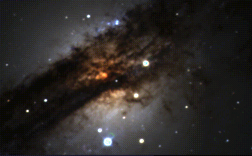
NGC 5128 host to SN 1986G is
an extremely peculiar and very
dusty galaxy. It is therefore difficult to properly de-redden the
SN light curve. For this reason, NGC 5128 is not used as a calibrator
even though it is the nearest galaxy (d
 3 Mpc) to host a SN Ia.
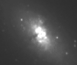
NGC 5253: This is a low mass
amorphous galaxy that has
hosted two SN Ia over the last 100 years (SN 1895B - see Schaefer
1995 for a recent analysis and SN 1972E). The occurrence of 2 SN Ia
in a galaxy of this low mass over the last 100 years is odd.
A distance modulus of (m - M) = 28.06 ± 0.06 mag has been determined
from measurements of eleven Cepheids by HST by Sandage et al. (1994).
IC 4182: This is another low
mass amorphous galaxy which
was the host of SN 1937C. Sandage et al. (1992) derive a distance based
on HST measurements of Cepheids.
These measurements, however, were made with the first Cycle of HST time
when the optics were not yet corrected for spherical aberration.
Concern has also been expressed about the reliability of the photographic
photometry of 1937C (see Pierce and Jacoby 1992).
| 
|
Figure 2-16 - 2-17: Images of the 2 nearby galaxies in which a SN Ia has occurred and which have Cepheid-based distance determinations. Top is a high contrast rendering of NGC 5253, in the red. This image is courtesy of Crystal Martin. The central region is dominated by blobs of star formation. The bottom image is of NGC 5128, courtesy of Bill Keel. NGC 5128 a famous galaxy noted for its very peculiar morphology. It has been suggested by many that this galaxy is a merger remnant. | |
The current calibration of the SN Ia distance scale is directly tied to the Cepheid distance scale. This allows for a consistency check if a supernova occurs in a nearby galaxy which has a Cepheid distance. This check is now available for the case of M100 which we discuss later in this chapter. The SN Ia luminosity calibration is uncertain due to errors in distance to these galaxies plus systematic error due to the adopted distances to the LMC or M31. Overall, however, the paucity of nearby calibrating SN Ia host galaxies is of real concern and raises the strong possibility of systematic bias, especially because the two calibrators are low mass, irregular galaxies and hence rather dissimilar to the host galaxies of more distant SN Ia. Very recently, Sandage et al. (1996) have added to the list of calibrating galaxies by including 3 in Virgo with Cepheid distances and the galaxy NGC 3627 in the Leo Group. We note that the distance moduli determined from Cepheids for the 3 Virgo spirals ranges from (m - M) = 31.10 ± 0.13 for NGC 4536 (Saha et al. 1996) to (m - M) = 32.0 for NGC 4639 (see Figure 2-18) (Sandage et al. 1996). We further note that Kennicutt et al. (1995) have identified 16 different papers in the recent literature that use the SN Ia distance scale to derive H0. These 16 papers yield a factor of 2 range in the value of H0 which almost certainly reflects 1) an insecure zeropoint for the method and 2) uncertainly in the correct calibration for the luminosity-decline relation.
|
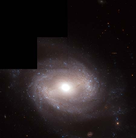
Figure 2-18: True-color CCD image obtained with the Hubble Space Telescope of NGC 4639. This spiral is located in the Virgo cluster and has hosted a Supernova Ia. Using HST a Cepheid distance to this galaxy has been determined by Sandage etal 1996. |
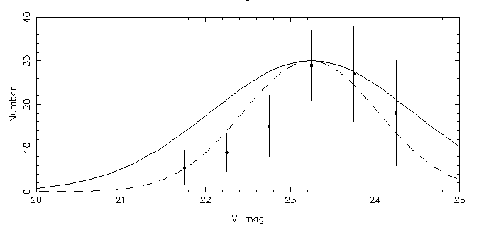
The Globular Cluster Luminosity Function
This is a population II distance indicator which rests on the assumption,
with very little a priori justification, that
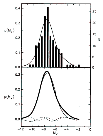
the Globular Cluster Luminosity Function (GCLF) is universal. For our galaxy,
the GCLF is Gaussian with a mean MV = -7.5 ± 0.2
and a dispersion
of 1.2 mag. This GCLF is
shown in Figure 2-19. Determining
the distance to an external galaxy involves measuring the peak
apparent magnitude of the GCLF. The method has the added advantage of being
relatively unaffected by reddening. The complications to this method
are the following:
The zeropoint of the
Galactic GCLF floats around by 0.3 mag depending
upon which sample of globular clusters with "good" distances is used.
For instance, Sandage and Tammann (1995) use MV = -7.6
± 0.1
for the Galaxy and MV = -7.7 ± 0.2 for M31
(using an M31 Cepheid
distance of (m - M) = 24.44). Abraham and van den Bergh (1995) derive
MV = -7.41 ± 0.11 for the Galaxy.
|
Figure 2-19: Representation of the GCLF for 136 Galactic Globular clusters from Abraham and van den Bergh (1995). They derive an absolute mean Visual mangitude of -7.41 with a disperion of 1.25 mag. |
In apparent magnitude space,
different galaxies exhibit different
Gaussian widths to their distribution and slightly different behavior at
the bright end of the LF. The different dispersions in the GCLFs may be
a population statistics effect and strongly indicate that the GCLF does
not have a uniform dispersion as is commonly assumed.
Figure 2-20 shows
the GCLF as determined for the galaxy NGC 7814 (see Bothun et al. 1992).
In this case, the observed
dispersion is significantly lower than the case for our Galaxy.
|
Figure 2-20: The CGLF as measured for NGC 7814 bu Bothun, Harris, and Hesser (1992). The dashed line is the best fit to the data and has a dispersion of 0.8 mag. The solid line represents a dispersion of 1.2 mag. |
Beyond a distance of 5 Mpc,
globular clusters can not
be detected individually and hence one relies on a statistical detection
of excess faint objects clustered around
a galaxy to define the Globular Cluster System (GCS) and hence the GCLF.
Most measured GCLFs are statistically determined.
In general, elliptical
galaxies have a richer GCS than do spirals,
yet it is the spiral GCLF which is used as the zeropoint. It is not
clear whether
the GCS of a spiral is a good analogue to that in an elliptical, especially if
some
ellipticals formed by mergers and the globular cluster themselves formed
in this
process (see Zepf et al. 1995).
However, there is some preliminary evidence that the GCLF does yield
consistent distances. For the ellipticals NGC 3379 and NGC 3377 (both
members of the
Leo group of galaxies), application of the GCLF
method gives (m - M) =
30.05 ±
0.40 (note the large error). Application of the PNLF method gives 29.9 and the
SBF method gives 29.7 for these two galaxies.
The above has summarized the 5 primary extragalactic distance indicators
which are currently used.
We do not include the Faber-Jackson method in this discussion. This
method, now modified to be the Dn -
 relation (see Dressler et al.
1987), is a dynamical method for
determining relative distances between elliptical galaxies, in a similar manner
that the TF relation is used for spiral galaxies. It is not included
in the present discussion because the relation has an unknown zeropoint. There
are no elliptical galaxies in the Local Group to calibrate it. The same
set of remarks apply to using the Brightest Cluster Member (BCM) as a
standard candle or using the "knee" of the galaxy luminosity function (see
Chapter 5). While they provide reasonable
estimates (maybe) of relative
distances between clusters, they can not be calibrated locally and hence
have no absolute zeropoint.
relation (see Dressler et al.
1987), is a dynamical method for
determining relative distances between elliptical galaxies, in a similar manner
that the TF relation is used for spiral galaxies. It is not included
in the present discussion because the relation has an unknown zeropoint. There
are no elliptical galaxies in the Local Group to calibrate it. The same
set of remarks apply to using the Brightest Cluster Member (BCM) as a
standard candle or using the "knee" of the galaxy luminosity function (see
Chapter 5). While they provide reasonable
estimates (maybe) of relative
distances between clusters, they can not be calibrated locally and hence
have no absolute zeropoint.