


In addition to temperature fluctuations, the simple physics of decoupling inevitably leads to non-zero polarization of the microwave background radiation as well, although quite generically the polarization fluctuations are expected to be significantly smaller than the temperature fluctuations. This section reviews the physics of polarization generation and its description. For a more detailed pedagogical discussion of microwave background polarization, see Kosowsky (1999), from which this section is excerpted.
Polarized light is conventionally described in terms of the Stokes parameters, which are presented in any optics text. If a monochromatic electromagnetic wave propogating in the z-direction has an electric field vector at a given point in space given by

| (10) |
then the Stokes parameters are defined as the following time averages:
| (11) |
| (12) |
| (13) |
| (14) |
The averages are over times long compared to the inverse frequency of the wave. The parameter I gives the intensity of the radiation which is always positive and is equivalent to the temperature for blackbody radiation. The other three parameters define the polarization state of the wave and can have either sign. Unpolarized radiation, or ``natural light,'' is described by Q = U = V = 0.
The parameters I and V are physical observables independent
of the coordinate system, but Q and U depend on the
orientation of the x and y axes. If a given wave is
described by the parameters Q and U for a certain
orientation of the coordinate system, then after a rotation of
the x - y plane through an angle
 , it is
straightforward to verify that the same wave is now
described by the parameters
, it is
straightforward to verify that the same wave is now
described by the parameters
| (15) |
From this transformation it is easy to see that the quantity
P2  Q2 + U2 is invariant under rotation
of the axes, and the angle
Q2 + U2 is invariant under rotation
of the axes, and the angle
| (16) |
defines a constant orientation parallel to the electric field of the wave. The Stokes parameters are a useful description of polarization because they are additive for incoherent superposition of radiation; note this is not true for the magnitude or orientation of polarization. Note that the transformation law in Eq. (15) is characteristic not of a vector but of the second-rank tensor

| (17) |
which also corresponds to the quantum mechanical
density matrix for an ensemble of photons
(Kosowsky 1996).
In kinetic theory, the photon distribution function
f (x, p, t) discussed in
Sec. 3.2 must
be generalized to
 ij(x,
p, t), corresponding to this density matrix.
ij(x,
p, t), corresponding to this density matrix.
4.2. Thomson scattering and the quadrupolar source
Non-zero linear polarization in the microwave background is generated around decoupling because the Thomson scattering which couples the radiation and the electrons is not isotropic but varies with the scattering angle. The total scattering cross-section, defined as the radiated intensity per unit solid angle divided by the incoming intensity per unit area, is given by
| (18) |
where  T is the total
Thomson cross section and
the vectors
T is the total
Thomson cross section and
the vectors
 and
' are unit
vectors in the planes perpendicular to the propogation directions
which are aligned with the outgoing and incoming polarization,
respectively. This scattering cross-section can give no net
circular polarization, so V = 0 for cosmological perturbations and
will not be discussed further. Measurements of V polarization can
be used as a diagnostic of systematic errors or microwave foreground
emission.
and
' are unit
vectors in the planes perpendicular to the propogation directions
which are aligned with the outgoing and incoming polarization,
respectively. This scattering cross-section can give no net
circular polarization, so V = 0 for cosmological perturbations and
will not be discussed further. Measurements of V polarization can
be used as a diagnostic of systematic errors or microwave foreground
emission.
It is a straightforward but slightly involved exercise to show that
the above relations imply that an incoming unpolarized radiation field
with the multipole expansion Eq. (6) incident
upon an electron in a sample volume with cross-section
B
will be Thomson scattered into an outgoing radiation field
from the sample volume with Stokes parameters
| (19) |
if the incoming radiation propagating in a given direction has rotational symmetry around its direction of propagation, as will hold for individual Fourier modes of scalar perturbations. Explicit expressions for the general case of no symmetry can be derived in terms of Wigner D-symbols (Kosowsky 1999).
In simple and general terms, unpolarized incoming radiation will be Thomson scattered into linearly polarized radiation if and only if the incoming radiation has a non-zero quadrupolar directional dependence. This single fact is sufficient to understand the fundamental physics behind polarization of the microwave background. During the tight-coupling epoch, the radiation field has only monopole and dipole directional dependences as explained above; therefore, scattering can produce no net polarization and the radiation remains unpolarized. As tight coupling begins to break down as recombination begins, a quadrupole moment of the radiation field will begin to grow due to free streaming of the photons. Polarization is generated during the brief interval when a significant quadrupole moment of the radiation has built up, but the scattering electrons have not yet all recombined. Note that if the universe recombined instantaneously, the net polarization of the microwave background would be zero. Due to this competition between the quadrupole source building up and the density of scatterers declining, the amplitude of polarization in the microwave background is generically suppressed by an order of magnitude compared to the temperature fluctuations.
Before polarization generation commences, the temperature fluctuations have either a monopole dependence, corresponding to density perturbations, or a dipole dependence, corresponding to velocity perturbations. A straightforward solution to the photon free-streaming equation (in terms of spherical Bessel functions) shows that for Fourier modes with wavelengths large compared to a characteristic thickness of the surface of last scattering, the quadrupole contribution through the last scattering surface is dominated by the velocity fluctuations in the temperature, not the density fluctuations. This makes intuitive sense: the dipole fluctuations can free stream directly into the quadrupole, but the monopole fluctuations must stream through the dipole first. This conclusion breaks down on small scales where either monopole or dipole can be the dominant quadrupole source, but numerical computations show that on scales of interest for microwave background fluctuations, the dipole temperature fluctuations are always the dominant source of quadrupole fluctuations at the surface of last scattering. Therefore, polarization fluctuations reflect mainly velocity perturbations at last scattering, in contrast to temperature fluctuations which predominantly reflect density perturbations.
4.3. Harmonic expansions and power spectra
Just as the temperature on the sky can be expanded into spherical harmonics, facilitating the computation of the angular power spectrum, so can the polarization. The situation is formally parallel, although in practice it is more complicated: while the temperature is a scalar quantity, the polarization is a second-rank tensor. We can define a polarization tensor with the correct transformation properties, Eq. (15), as
| (20) |
The dependence on the Stokes parameters is the same as for the density matrix, Eq. 17; the extra factors are convenient because the usual spherical coordinate basis is orthogonal but not orthonormal. This tensor quantity must be expanded in terms of tensor spherical harmonics which preserve the correct transformation properties. We assume a complete set of orthonormal basis functions for symmetric trace-free 2 × 2 tensors on the sky,
| (21) |
where the expansion coefficients are given by
| (22) |
| (23) |
which follow from the orthonormality properties

| (24) |
| (25) |
These tensor spherical harmonics are not as exotic as they might sound; they are used extensively in the theory of gravitational radiation, where they naturally describe the radiation multipole expansion. Tensor spherical harmonics are similar to vector spherical harmonics used to represent electromagnetic radiation fields, familiar from Chapter 16 of Jackson (1975). Explicit formulas for tensor spherical harmonics can be derived via various algebraic and group theoretic methods; see Thorne (1980) for a complete discussion. A particularly elegant and useful derivation of the tensor spherical harmonics (along with the vector spherical harmonics as well) is provided by differential geometry: the harmonics can be expressed as covariant derivatives of the usual spherical harmonics with respect to an underlying manifold of a two-sphere (i.e., the sky). This construction has been carried out explicitly and applied to the microwave background polarization (Kamionkowski, Kosowsky, and Stebbins 1996).
The existence of two sets of basis functions, labeled here by ``G''
and ``C'', is due to the fact that the symmetric traceless 2 × 2
tensor describing linear polarization is specified by two independent
parameters. In two dimensions, any symmetric traceless tensor can be
uniquely decomposed into a part of the form
A;ab -
(1/2)gabA;cc and another
part of the form B;ac
 cb +
B;bc
ca
where A and B are
two scalar functions and semicolons indicate covariant derivatives. This
decomposition is quite similar to the decomposition of a vector field
into a part which is the gradient of a scalar field and a part which
is the curl of a vector field; hence we use the notation G for
``gradient'' and C for ``curl''. In fact, this correspondence is more
than just cosmetic: if a linear polarization field is visualized in
the usual way with headless ``vectors'' representing the amplitude and
orientation of the polarization, then the G harmonics describe the
portion of the polarization field which has no handedness associated
with it, while the C harmonics describe the other portion of the field
which does have a handedness (just as with the gradient and curl of a
vector field). Note that
Zaldarriaga and
Seljak (1997)
label these harmonics E and B, with a slightly different normalization than
defined here (see
Kamionkowski et al. 1996).
cb +
B;bc
ca
where A and B are
two scalar functions and semicolons indicate covariant derivatives. This
decomposition is quite similar to the decomposition of a vector field
into a part which is the gradient of a scalar field and a part which
is the curl of a vector field; hence we use the notation G for
``gradient'' and C for ``curl''. In fact, this correspondence is more
than just cosmetic: if a linear polarization field is visualized in
the usual way with headless ``vectors'' representing the amplitude and
orientation of the polarization, then the G harmonics describe the
portion of the polarization field which has no handedness associated
with it, while the C harmonics describe the other portion of the field
which does have a handedness (just as with the gradient and curl of a
vector field). Note that
Zaldarriaga and
Seljak (1997)
label these harmonics E and B, with a slightly different normalization than
defined here (see
Kamionkowski et al. 1996).
We now have three sets of multipole moments, a(lm)T, a(lm)G, and a(lm)C, which fully describe the temperature/polarization map of the sky. These moments can be combined quadratically into various power spectra analogous to the temperature ClT. Statistical isotropy implies that
| (26) |
where the angle brackets are an average over all realizations of the probability distribution for the cosmological initial conditions. Simple statistical estimators of the various Cl's can be constructed from maps of the microwave background temperature and polarization.
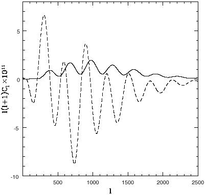
For fluctuations with gaussian random distributions (as predicted by the simplest inflation models), the statistical properties of a temperature/polarization map are specified fully by these six sets of multipole moments. In addition, the scalar spherical harmonics Y(lm) and the G tensor harmonics Y(lm)abG have parity (- 1)l, but the C harmonics Y(lm)abC have parity (- 1)l + 1. If the large-scale perturbations in the early universe were invariant under parity inversion, then ClTC = ClGC = 0. So generally, microwave background fluctuations are characterized by the four power spectra ClT, ClG, ClC, and ClTG. These The end result of the numerical computations described in Sec. 3.2 above are these power spectra. Polarization power spectra ClG and ClTG for scalar perturbations in a typical inflation-like cosmological model, generated with the CMBFAST code (Seljak and Zaldarriaga 1996), are displayed in Fig. 2. The temperature power spectrum in Fig. 1 and the polarization power spectra in Fig. 2 come from the same cosmological model. The physical source of the features in the power spectra is discussed in the next section, followed by a discussion of how cosmological parameters can be determined to high precision via detailed measurements of the microwave background power spectra.
|
Figure 2. The G polarization power spectrum (solid line) and the cross-power TG between temperature and polarization (dashed line), for the same model as in Fig. 1. |