


2.3 The Gaussian or Normal Distribution
The Gaussian or normal distribution plays a central role in all of statistics and is the most ubiquitous distribution in all the sciences. Measurement errors, and in particular, instrumental errors are generally described by this probability distribution. Moreover, even in cases where its application is not strictly correct, the Gaussian often provides a good approximation to the true governing distribution.
The Gaussian is a continuous, symmetric distribution whose density is given by
The two parameters µ and
Fig. 3. The Gaussian distribution for various
The shape of the Gaussian is shown in Fig. 3
which illustrates this distribution for various
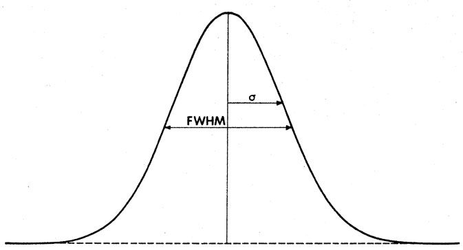
This is illustrated in Fig. 4. In such cases,
care should be taken
to be clear about which parameter is being used. Another width
parameter which is also seen in the Literature is the full-width at
one-tenth maximum (FWTM).
Fig. 4. Relation between the standard
deviation a and the full width at half-maximum (FWHM).
The integral distribution for the Gaussian density, unfortunately,
cannot be calculated analytically so that one must resort to numerical
integration. Tables of integral values are readily found as
well. These are tabulated in terms of a reduced Gaussian distribution
with µ = 0 and
where µ and
Fig. 5. The area contained between the
limits µ ± 1
An important practical note is the area under the Gaussian between
integral intervals of
 2 can be shown to
correspond to the mean and
variance of the distribution by applying (8) and (9).
2 can be shown to
correspond to the mean and
variance of the distribution by applying (8) and (9).
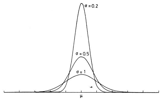
. The standard
deviation determines the width of the distribution.
. The significance of
as a measure of
the distribution width is clearly seen. As can be calculated from
(19), the standard deviation corresponds to the half width of the
peak at about 60% of the full height. In some applications, however,
the full width at half maximum (FWHM) is often used instead. This is
somewhat larger than and can
easily be shown to be
2 = 1. All Gaussian
distributions may be transformed
to this reduced form by making the variable transformation
 are
the mean and standard deviation of the original
distribution. It is a trivial matter then to verify that z is
distributed as a reduced Gaussian.
are
the mean and standard deviation of the original
distribution. It is a trivial matter then to verify that z is
distributed as a reduced Gaussian.

,
µ ± 2 and
µ ± 3
in a Gaussian distribution.
. This is
shown in Fig. 5. These values
should be kept in mind when interpreting measurement errors. The
presentation of a result as x ±
signifies, in fact, that the true
value has  68% probability of
lying between the limits x -
and x +
or a 95% probability of lying
between x - 2 and
x + 2, etc. Note
that for a 1 interval, there is
almost a 1/3 probability that the
true value is outside these limits! If two standard deviations are
taken, then, the probability of being outside is only
5%, etc.
68% probability of
lying between the limits x -
and x +
or a 95% probability of lying
between x - 2 and
x + 2, etc. Note
that for a 1 interval, there is
almost a 1/3 probability that the
true value is outside these limits! If two standard deviations are
taken, then, the probability of being outside is only
5%, etc.