


Some theoretical background of radio radiation, interferometry and receiver technology has been given in G. Miley's contribution to these proceedings. In this section I shall briefly compare the advantages and limitations of both single dishes and radio interferometers, and mention some tools to overcome or alleviate some of their limitations. For a discussion of various types of radio telescopes see [Christiansen & Högbom (1985)]. Here I limit myself to those items which appear most important to take into account when trying to make use of, and to interpret, radio maps drawn from public archives.
2.1. Single Dishes versus Interferometers
The basic relation between the angular resolution
 and the
aperture (or diameter) D of a telescope is
and the
aperture (or diameter) D of a telescope is

 / D radians, where
is the wavelength of
observation. For the radio domain
is ~ 106 times
larger than in the optical, which would imply that one has to build a
radio telescope a million times larger than an optical
one to obtain the same angular resolution. In the early days of radio
astronomy, when the observing equipment was based on radar dishes
no longer required by the military after World War II,
typical angular resolutions achieved were of the order of degrees.
Consequently interferometry developed into an important and successful
technique by the early 1950s (although arrays of dipoles, or Yagi
antennas were used, rather than parabolic dishes, because the
former were more suited to the metre-wave band used in the early
experiments). Improved economic conditions and
technological advance also permitted a significant increase in the size
of single dishes. However, the sheer weight of the reflector and its support
structure has set a practical limit of about 100 metres for fully steerable
parabolic single dishes. Examples are the Effelsberg 100-m dish
(www.mpifr-bonn.mpg.de/index_e.html) near
Bad Münstereifel in Germany, completed in 1972, and the
Green Bank Telescope (GBT; Section 8) in West
Virginia, USA, to be
completed in early 2000. The spherical 305-m antenna near Arecibo
(Puerto Rico; www.naic.edu/)
is the largest single dish
available at present. However, it is not steerable; it is built in
a natural and close-to-spherical depression in the ground, and has a limiting
angular resolution of ~ 1' at the highest operating frequency (8GHz).
Apart from increasing the dish size, one may also increase the observing
frequency to improve the angular resolution. However, the D in the above
formula is the aperture within which the antenna surface is accurate to
better than ~ 0.1 , and the
technical
limitations imply that the bigger the antenna, the less accurate the surface.
In practice this means that a single dish never achieves a resolution
of better than ~ 10"-20", even at sub-mm wavelengths
(cf. Fig. 6.8 in
[Rohlfs &
Wilson (1996)]).
/ D radians, where
is the wavelength of
observation. For the radio domain
is ~ 106 times
larger than in the optical, which would imply that one has to build a
radio telescope a million times larger than an optical
one to obtain the same angular resolution. In the early days of radio
astronomy, when the observing equipment was based on radar dishes
no longer required by the military after World War II,
typical angular resolutions achieved were of the order of degrees.
Consequently interferometry developed into an important and successful
technique by the early 1950s (although arrays of dipoles, or Yagi
antennas were used, rather than parabolic dishes, because the
former were more suited to the metre-wave band used in the early
experiments). Improved economic conditions and
technological advance also permitted a significant increase in the size
of single dishes. However, the sheer weight of the reflector and its support
structure has set a practical limit of about 100 metres for fully steerable
parabolic single dishes. Examples are the Effelsberg 100-m dish
(www.mpifr-bonn.mpg.de/index_e.html) near
Bad Münstereifel in Germany, completed in 1972, and the
Green Bank Telescope (GBT; Section 8) in West
Virginia, USA, to be
completed in early 2000. The spherical 305-m antenna near Arecibo
(Puerto Rico; www.naic.edu/)
is the largest single dish
available at present. However, it is not steerable; it is built in
a natural and close-to-spherical depression in the ground, and has a limiting
angular resolution of ~ 1' at the highest operating frequency (8GHz).
Apart from increasing the dish size, one may also increase the observing
frequency to improve the angular resolution. However, the D in the above
formula is the aperture within which the antenna surface is accurate to
better than ~ 0.1 , and the
technical
limitations imply that the bigger the antenna, the less accurate the surface.
In practice this means that a single dish never achieves a resolution
of better than ~ 10"-20", even at sub-mm wavelengths
(cf. Fig. 6.8 in
[Rohlfs &
Wilson (1996)]).
Single dishes do not offer the possibility of instantaneous imaging as with interferometers by Fourier transform of the visibilities. Instead, several other methods of observation can be used with single dishes. If one is interested merely in integrated parameters (flux, polarisation, variability) of a (known) point source, one can use ``cross-scans'' centred on the source. If one is very sure about the size and location of the source (and its neighbourhood) one can even use ``on-off'' scans, i.e. point on the source for a while, then point to a neighbouring patch of ``empty sky'' for comparison. This is usually done using a pair of feeds and measuring their difference signal. However, to take a real image with a single dish it is necessary to raster the field of interest, by moving the telescope e.g. along right ascension (RA), back and forth, each scan shifted in declination (DEC) with respect to the other by an amount of no more than ~ 40% of the half-power beam width (HPBW) if the map is to be fully sampled. At decimetre wavelengths this has the advantage of being able to cover a much larger area than with a single ``pointing'' of an interferometer (unless the interferometer elements are very small, thus requiring large amounts of integration time). The biggest advantage of this raster method is that it allows the map size to be adjusted to the size of the source of interest, which can be several degrees in the case of large radio galaxies or supernova remnants (SNRs). Using this technique a single dish is capable of tracing (in principle) all large-scale features of very extended radio sources. One may say that it ``samples'' spatial frequencies in a range from the the map size down to the beam width. This depends critically on the way in which a baseline is fitted to the individual scans. The simplest way is to assume the absence of sources at the map edges, set the intensity level to zero there, and interpolate linearly between the two opposite edges of the map. A higher-order baseline is able to remove the variable atmospheric effects more efficiently, but it may also remove real underlying source structure. For example, the radio extent of a galaxy may be significantly underestimated if the map was made too small. Rastering the galaxy in two opposite directions may help finding emission close to the map edges using the so-called ``basket-weaving'' technique ([Sieber et al. (1979)]). Different methods in baseline subtraction and cut-offs in source size have led to two different versions of source catalogues ([Becker et al. (1991)] and [Gregory & Condon (1991)]), both drawn from the 4.85-GHz Green Bank survey. The fact that the surface density of these sources does not change towards the Galactic plane, while in the very similar southern PMN survey ([Tasker & Wright (1993)]) it does, is entirely due to differences in the data reduction method (Section 3.3).
In contrast to single dishes, interferometers often have excellent
angular resolution (again
/ D,
but now D is the maximum distance between any pair of antennas
in the array). However, the field of view is
FOV
/ d, where
d is the size of an individual antenna.
Thus, the smaller the individual antennas, the larger the field of view,
but also the worse the sensitivity. Very large numbers of antennas increase
the design cost for the array and the on-line correlator to process
the signals from a large number of interferometer pairs.
An additional aspect of interferometers is their reduced
sensitivity to extended source components, which depends essentially
on the smallest distance, say
Dmin, between two antennas in
the interferometer array. This is often called the minimum spacing or
shortest baseline. Roughly speaking, source components
larger than ~ /
Dmin radians will be attenuated
by more than 50% of their flux, and thus practically be lost.
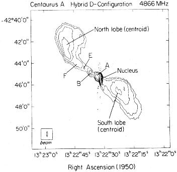
Figure 1 gives an extreme example of this,
showing two images of the radio galaxy with the largest apparent size
in the sky (10°). It is instructive to compare this with
a high-frequency single-dish map in
[Junkes et al. (1993)].

| 
|
Figure 1. Map of the Centaurus A region from the 408MHz all-sky survey (Haslam et al. (1981), showing the full north-south extent of ~ 10° of the radio structure and an emission feature due south east, apparently ``connecting'' Cen A with the plane of our Galaxy (see Combi et al. 1998). Right: A 1.4GHz map obtained with the VLA (from Burns et al. 1983) showing the inner 10' of Cen A. Without a single-dish map the full size of Cen Ae would not have been recognised. | |
The limitation in sensitivity for extended structure is even more severe for Very Long Baseline Interferometry (VLBI) which uses intercontinental baselines providing ~ 10-3 arcsec (1 mas) resolution. The minimum baseline is often several hundred km, making the largest detectable component much smaller than an arcsec.
[McKay & McKay (1998)] created a WWW tool that simulates how radio interferometers work. This Virtual Radio Interferometer (VRI; www.jb.man.ac.uk/~dm/vri/) comes with the ``VRI Guide'' describing the basic concepts of radio interferometry. The applet simulates how the placement of the antennas affects the uv-coverage of a given array and illustrates the Fourier transform relationship between the accumulated radio visibilities and the resultant image.
The comparatively low angular resolution of single dish radio telescopes naturally suggests their use at relatively high frequencies. However, at centimetre wavelengths atmospheric effects (e.g. passing clouds) will introduce additional emission or absorption while scanning, leaving a stripy pattern along the scanning direction (so-called ``scanning effects''). Rastering the same field along DEC rather than RA, would lead to a pattern perpendicular to the first one. A comparison and subsequent combination of the two maps, either in the real or the Fourier plane, can efficiently suppress these patterns and lead to a sensitive map of the region ([Emerson & Gräve (1988)]).
A further efficient method to reduce atmospheric effects in single-dish radio maps is the so-called ``multi-feed technique''. The trick is to use pairs of feeds in the focal plane of a single dish. At any instant each feed receives the emission from a different part of the sky (their angular separation, or ``beam throw'', is usually 5-10 beam sizes). Since they largely overlap within the atmosphere, they are affected by virtually the same atmospheric effects, which then cancel out in the difference signal between the two feeds. The resulting map shows a positive and negative image of the same source, but displaced by the beam throw. This can then be converted to a single positive image as described in detail by [Emerson et al. (1979)]. One limitation of the method is that source components larger than a few times the largest beam throw involved will be lost. The method has become so widely used that an entire symposium has been dedicated to it ([Emerson & Payne (1995)]).
From the above it should be clear that single dishes and interferometers actually complement each other well, and in order to map both the small- and large-scale structures of a source it may be necessary to use both. Various methods for combining single-dish and interferometer data have been devised, and examples of results can be found in [Brinks & Shane (1984)], [Landecker et al. (1990)], [Joncas et al. (1992)], Landecker et al. (1992), [Normandeau et al. (1992)] or [Langer et al. (1995)]. The Astronomical Image Processing System (AIPS; www.cv.nrao.edu/aips), a widely used reduction package in radio astronomy, provides the task IMERG (cf. www.cv.nrao.edu/aips/cook.html) for this purpose. The software package Miriad (www.atnf.csiro.au/computing/software/miriad) for reduction of radio interferometry data offers two programs (immerge and mosmem) to realise this combination of single dish and interferometer data (Section 2.3). The first one works in the Fourier plane and uses the single dish and mosaic data for the short and long spacings, respectively. The second one compares the single dish and mosaic images and finds the ``Maximum Entropy'' image consistent with both.
2.2. Special Techniques in Radio Interferometry
A multitude of ``cosmetic treatments'' of interferometer data have been developed, both for the ``uv-'' or visibility data and for the maps (i.e. before and after the Fourier transform), mostly resulting from 20 years of experience with the most versatile and sensitive radio interferometers currently available, the Very Large Array (VLA) and its more recent VLBI counterparts the European VLBI Network (EVN), and the Very Large Baseline Array (VLBA); see their WWW pages at www.nrao.edu/vla/html/VLAhome.shtml, www.nfra.nl/jive/evn/evn.html, and www.nrao.edu/vlba/html/VLBA.html. The volumes edited by [Perley et al. (1989), Cornwell & Perley (1991)], and [Zensus et al. (1995)] give an excellent introduction to these effects, the procedures for treating them, as well as their limitations. The more prominent topics are bandwidth and time-average smearing, aliasing, tapering, uv-filtering, CLEANing, self-calibration, spectral-line imaging, wide-field imaging, multi-frequency synthesis, etc.
One way to extend the field of view of interferometers is to take ``snapshots'' of several individual fields with adjacent pointing centres (or phase centres) spaced by no further than about one (and preferably half a) ``primary beam'', i.e. the HPBW of the individual array element. For sources larger than the primary beam of the single interferometer elements the method recovers interferometer spacings down to about half a dish diameter shorter than those directly measured, while for sources that fit into the primary beam mosaicing (also spelled ``mosaicking'') will recover spacings down to half the dish diameter ([Cornwell (1988)], or [Cornwell (1989)]). The data corresponding to shorter spacings can be taken either from other single-dish observations, or from the array itself, using it in a single-dish mode. The ``Berkeley Illinois Maryland Association'' (BIMA; bima.astro.umd.edu/bima/) has developed a homogeneous array capability, which is the central design issue for the planned NRAO Millimeter Array (MMA; www.mma.nrao.edu/). The strategy involves mosaic observations with the BIMA compact array during a normal 6-8 hour track, coupled with single-antenna observations with all array antennas mapping the same extended field (see [Pound et al. (1997)] or bima.astro.umd.edu:80/bima/memo/memo57.ps).
Approximately 15% of the observing time on the Australia Telescope Compact Array (ATCA; www.narrabri.atnf.csiro.au/) is spent on observing mosaics. A new pointing centre may be observed every 25 seconds, with only a few seconds of this time consumed by slewing and other overheads. The largest mosaic produced on the ATCA by 1997 is a 1344 pointing-centre spectral-line observation of the Large Magellanic Cloud. Joint imaging and deconvolution of this data produced a 1997 × 2230 × 120 pixel cube (see www.atnf.csiro.au/research/lmc_h1/). Mosaicing is heavily used in the current large-scale radio surveys like NVSS, FIRST, and WENSS (Section 3.7).
The dynamic range of a map is usually defined as the ratio of the peak brightness to that of the ``lowest reliable brightness level'', or alternatively to that of the rms noise of a source-free region of the image. For both interferometers and single dishes the dynamic range is often limited by sidelobes occurring near strong sources, either due to limited uv-coverage, and/or as part of the diffraction pattern of the antenna. Sometimes the dynamic range, but more often the ratio between the peak brightness of the sidelobe and the peak brightness of the source, is given in dB, this being ten times the decimal logarithm of the ratio. In interferometer maps these sidelobes can usually be reduced using the CLEAN method, although more sophisticated methods are required for the strongest sources (cf. [Noordam & deBruyn (1982)], [Perley (1989)]), for which dynamic ranges of up to 5 × 10⁵ can be achieved ([deBruyn & Sijbring (1993)]). For an Alt-Az single dish the sidelobe pattern rotates with time on the sky, so a simple average of maps rastered at different times can reduce the sidelobe level. But again, to achieve dynamic ranges of better than a few thousand the individual scans have to be corrected independently before they can be averaged ([Klein & Mack (1995)]).
Confusion occurs when there is more than one source in the
telescope beam. For a beam area
 b, the confusion
limit Sc is the flux density at which this happens as one
considers fainter and fainter sources. For an integral source count
N(S), i.e. the number of sources per sterad brighter than flux density
S, the number of sources in a telescope beam
b is
b N(S).
Sc is then given by
b
N(Sc)
1. A radio survey is
said to be confusion-limited if the expected minimum detectable
flux density
Smin is lower than Sc. Clearly, the confusion limit
decreases with increasing observing frequency and with smaller telescope
beamwidth. Apart from estimating the confusion limit theoretically from
source counts obtained with a telescope of much lower confusion level
(see [Condon (1974)]),
one can also derive the confusion limit empirically by subsequent
weighted averaging of N maps with (comparable) noise level
b, the confusion
limit Sc is the flux density at which this happens as one
considers fainter and fainter sources. For an integral source count
N(S), i.e. the number of sources per sterad brighter than flux density
S, the number of sources in a telescope beam
b is
b N(S).
Sc is then given by
b
N(Sc)
1. A radio survey is
said to be confusion-limited if the expected minimum detectable
flux density
Smin is lower than Sc. Clearly, the confusion limit
decreases with increasing observing frequency and with smaller telescope
beamwidth. Apart from estimating the confusion limit theoretically from
source counts obtained with a telescope of much lower confusion level
(see [Condon (1974)]),
one can also derive the confusion limit empirically by subsequent
weighted averaging of N maps with (comparable) noise level
 i,
and with each of them not confusion-limited. The weight of each map
should be proportional to
i-2.
In the absence of confusion, the expected noise,
N,exp, of the
average map should then be
i,
and with each of them not confusion-limited. The weight of each map
should be proportional to
i-2.
In the absence of confusion, the expected noise,
N,exp, of the
average map should then be
|
If this is confirmed by experiment, we can say that the ``confusion noise''
is negligible, or at least that
c <<
N. However,
if N approaches a
saturation limit with increasing N, then the confusion noise,
c, can be
estimated according to
c2 =
obs2 -
N,exp2.
As an example, the confusion limit of a 30-m dish at 1.5GHz
( = 20cm)
and a beam width of HPBW = 34' is ~ 400mJy. For a 100-m telescope
at 2.7, 5 and 10.7GHz ( =
11cm, 6cm and 2.8cm;
HPBW = 4.4', 2.5' and 1.2'), the confusion limits are ~ 2, 0.5, and
 0.1mJy. For
the VLA D-array at 1.4GHz (HPBW = 50") it is ~ 0.1mJy.
For radio interferometers the confusion noise is generally
negligible owing to their high angular resolution, except for deep
maps at low frequencies where confusion due to sidelobes becomes
significant (e.g. for WENSS and SUMSS, see
Section 3.7).
Note the semantic difference
between ``confusion noise'' and ``confusion limit''. They can be related
by saying that in a confusion-limited survey, point sources can be
reliably detected only above the confusion limit, or 2-3 times the
confusion noise, while coherent extended structures can be reliably
detected down to lower limits, e.g. by convolution of the map to lower
angular resolution. There is virtually no confusion limit for
polarised intensity, as the polarisation position angles of
randomly distributed, faint background sources tend to cancel out
any net polarisation (see
[Rohlfs & Wilson
(1996)],
p.216 for more details).
Examples of confusion-limited surveys are the large-scale
low frequency surveys e.g. at 408MHz
([Haslam et al. (1982)]),
at 34.5MHz
([Dwarakanath & Udaya Shankar (1990)]),
and at 1.4GHz
([Condon & Broderick (1986a)]).
Of course, confusion
becomes even more severe in crowded areas like the Galactic plane
([Kassim (1988)]).
0.1mJy. For
the VLA D-array at 1.4GHz (HPBW = 50") it is ~ 0.1mJy.
For radio interferometers the confusion noise is generally
negligible owing to their high angular resolution, except for deep
maps at low frequencies where confusion due to sidelobes becomes
significant (e.g. for WENSS and SUMSS, see
Section 3.7).
Note the semantic difference
between ``confusion noise'' and ``confusion limit''. They can be related
by saying that in a confusion-limited survey, point sources can be
reliably detected only above the confusion limit, or 2-3 times the
confusion noise, while coherent extended structures can be reliably
detected down to lower limits, e.g. by convolution of the map to lower
angular resolution. There is virtually no confusion limit for
polarised intensity, as the polarisation position angles of
randomly distributed, faint background sources tend to cancel out
any net polarisation (see
[Rohlfs & Wilson
(1996)],
p.216 for more details).
Examples of confusion-limited surveys are the large-scale
low frequency surveys e.g. at 408MHz
([Haslam et al. (1982)]),
at 34.5MHz
([Dwarakanath & Udaya Shankar (1990)]),
and at 1.4GHz
([Condon & Broderick (1986a)]).
Of course, confusion
becomes even more severe in crowded areas like the Galactic plane
([Kassim (1988)]).
When estimating the error in flux density of sources (or their
significance) several factors have to be taken into account.
The error in absolute calibration,
 cal, depends on the
accuracy of the adopted flux density scale and is usually of the order
of a few per cent. Suitable absolute calibration sources for single-dish
observations are listed in
[Baars et al. (1977)] and
[Ott et al. (1994)]
for intermediate frequencies, and in
[Rees (1990a)]
for low frequencies. Note that
for the southern hemisphere older flux scales are still in use, e.g.
[Wills (1975)].
Lists of calibrator sources for intermediate-resolution interferometric
observations (such as the VLA) can be found at the URL
www.nrao.edu/~gtaylor/calib.html, and those for very-high
resolution observations (such as the VLBA) at
magnolia.nrao.edu/vlba_calib/vlbaCalib.txt.
When comparing different source lists it is important to note that,
especially at frequencies below ~ 400MHz, there are still different
``flux scales'' being used which may differ by
cal, depends on the
accuracy of the adopted flux density scale and is usually of the order
of a few per cent. Suitable absolute calibration sources for single-dish
observations are listed in
[Baars et al. (1977)] and
[Ott et al. (1994)]
for intermediate frequencies, and in
[Rees (1990a)]
for low frequencies. Note that
for the southern hemisphere older flux scales are still in use, e.g.
[Wills (1975)].
Lists of calibrator sources for intermediate-resolution interferometric
observations (such as the VLA) can be found at the URL
www.nrao.edu/~gtaylor/calib.html, and those for very-high
resolution observations (such as the VLBA) at
magnolia.nrao.edu/vlba_calib/vlbaCalib.txt.
When comparing different source lists it is important to note that,
especially at frequencies below ~ 400MHz, there are still different
``flux scales'' being used which may differ by
 10%,
and even more below ~ 100MHz.
The ``zero-level error'' is important mainly for single-dish
maps and is given by
° =
m
10%,
and even more below ~ 100MHz.
The ``zero-level error'' is important mainly for single-dish
maps and is given by
° =
m
 n,
where m is the number of beam areas contained in the source
integration area,
n is the number of beam areas in the area of noise determination, and
is the noise level
determined in regions ``free of emission''
(and includes contributions from the receiver, the atmosphere,
and confusion). The error due to noise in the integration area
is =
m .
The three errors combine to give a total flux density error of
(see [Klein & Emerson (1981))
S =
cal +
sqrt[°2 +
2] .
Clearly, the relative error grows with the extent of a source. This also
implies that the upper limit to the flux density of a non-detected source
depends on the size assumed for it: while a point source of ten times the
noise level will clearly be detected, a source of the same flux, but
extending over many antenna beams may well remain undetected.
In interferometer observations the non-zero size of the shortest baseline
limits the sensitivity to extended sources. At frequencies
10GHz the atmospheric
absorption starts to
become important, and the measured flux S will depend on elevation
n,
where m is the number of beam areas contained in the source
integration area,
n is the number of beam areas in the area of noise determination, and
is the noise level
determined in regions ``free of emission''
(and includes contributions from the receiver, the atmosphere,
and confusion). The error due to noise in the integration area
is =
m .
The three errors combine to give a total flux density error of
(see [Klein & Emerson (1981))
S =
cal +
sqrt[°2 +
2] .
Clearly, the relative error grows with the extent of a source. This also
implies that the upper limit to the flux density of a non-detected source
depends on the size assumed for it: while a point source of ten times the
noise level will clearly be detected, a source of the same flux, but
extending over many antenna beams may well remain undetected.
In interferometer observations the non-zero size of the shortest baseline
limits the sensitivity to extended sources. At frequencies
10GHz the atmospheric
absorption starts to
become important, and the measured flux S will depend on elevation
 approximately according
to S = S° exp(-
approximately according
to S = S° exp(- csc ),
where S° is the extra-atmospheric flux density, and
the
optical depth of the atmosphere.
E.g., at 10.7GHz and at sea level, typical values of
are
0.05-0.10, i.e. 5-10% of the flux is absorbed even
when pointing at the zenith. These increase with frequency, but decrease
with altitude of the observatory.
Uncertainties in the zenith-distance dependence
may well dominate other sources of error above ~ 50GHz.
csc ),
where S° is the extra-atmospheric flux density, and
the
optical depth of the atmosphere.
E.g., at 10.7GHz and at sea level, typical values of
are
0.05-0.10, i.e. 5-10% of the flux is absorbed even
when pointing at the zenith. These increase with frequency, but decrease
with altitude of the observatory.
Uncertainties in the zenith-distance dependence
may well dominate other sources of error above ~ 50GHz.
When estimating flux densities from interferometer maps, the maps should have been corrected for the polar diagram (or ``primary beam'') of the individual antennas, which implies a decreasing sensitivity with increasing distance from the pointing direction. This so-called ``primary-beam correction'' divides the map by the attenuation factor at each map point and thus raises both the intensity of sources, and the map noise, with increasing distance from the phase centre. Some older source catalogues, mainly obtained with the Westerbork Synthesis Radio Telescope (WSRT; e.g. [Oort & vanLangevelde (1987)], or [Righetti et al. (1988)]) give both the (uncorrected) ``map flux'' and the (primary-beam corrected) ``sky flux''. The increasing uncertainty of the exact primary beam shape with distance from the phase centre may dominate the flux density error on the periphery of the field of view.
Care should be taken in the
interpretation of structural source parameters in catalogues.
Some catalogues list the ``map-fitted'' source size,
m ,
as drawn directly from a Gaussian fit of the map. Others quote
the ``deconvolved'' or ``intrinsic'' source size,
s .
All of these are model-dependent and usually assume both the source and
the telescope beam to be Gaussian (with full-width at half maximum,
FWHM = b), in
which case we have
b2 +
s2 =
m2
Values of ``0.0'' in the size column of catalogues are often found for
``unresolved'' sources. Rather than zero, the intrinsic size is smaller
than a certain fraction of the telescope beam width. The fraction
decreases with increasing signal-to-noise (S/N) ratio of the source.
Estimation of errors in the structure parameters derived from
2-dimensional radio maps is discussed in
[Condon (1997)].
Sometimes flux densities are quoted which are smaller than the error,
or even negative (e.g.
[Dressel & Condon (1978)], and
[Klein et al. (1996)]).
These should actually be converted to,
and interpreted as upper limits to the flux density.
2.5. Intercomparison of Different Observations and Pitfalls
Two main emission mechanisms are at work in radio sources (e.g. [Pacholczyk (1970)]). The non-thermal synchrotron emission of relativistic electrons gyrating in a magnetic field is responsible for supernova remnants, the jets and lobes of radio galaxies and much of the diffuse emission in spiral galaxies (including ours) and their haloes. The thermal free-free or bremsstrahlung of an ionised gas cloud dominates e.g. in HII regions, planetary nebulae, and in spiral galaxies at high radio frequencies. In addition, individual stars may show ``magneto-bremsstrahlung'', which is synchrotron emission from either mildly relativistic electrons (``gyrosynchrotron'' emission) or from less relativistic electrons (``cyclotron'' or ``gyroresonance'' emission). The historical confirmation of synchrotron radiation came from the detection of its polarisation. In contrast, thermal radiation is unpolarised, and characterised by a very different spectral shape than that of synchrotron radiation. Thus, in order to distinguish between these mechanisms, multi-frequency comparisons are needed. This is trivial for unresolved sources, but for extended sources care has to be taken to include the entire emission, i.e. integrated over the source area. Peak fluxes or fluxes from high-resolution interferometric observations will usually underestimate their total flux. Very-low frequency observations may overestimate the flux by picking up radiation from neighbouring (or ``blending'') sources within their wide telescope beams. Compilations of integrated spectra of large numbers of extragalactic sources have been prepared e.g. by [Kühr et al. (1979)], [Herbig & Readhead (1992)], and [Bursov et al. (1997)] (see cats.sao.ru/cats_spectra.html).
An important diagnostic of the energy transfer within radio sources is a two-dimensional comparison of maps observed at different frequencies. Ideally, with many such frequencies, a spectral fit can be made at each resolution element across the source and parameters like the relativistic electron density and radiation lifetime, magnetic field strength, separation of thermal and non-thermal contribution, etc. can be estimated (cf. [Klein et al. (1989)] or [Katz-Stone & Rudnick (1994)]). However, care must be taken that the observing instruments at the different frequencies were sensitive to the same range of ``spatial frequencies'' present in the source. Thus interferometer data which are to be compared with single-dish data should be sensitive to components comparable to the entire size of the source. The VLA has a set of antenna configurations with different baseline lengths that can be matched to a subset of observing frequencies in order to record a similar set of spatial frequencies at widely different wavelengths - these are called ``scaled arrays''. For example, the B-configuration at 1.4GHz and the C-configuration at 4.8GHz form one such pair of arrays. Recent examples of such comparisons for very extended radio galaxies can be found in [Mack et al. (1997)] or [Sijbring & deBruyn (1998)]. Maps of the spectral indices of Galactic radio emission between 408 and 1420MHz have even been prepared for the entire northern sky ([Reich & Reich (1988)]). Here the major limitation is the uncertainty in the absolute flux calibration.
2.6. Linear Polarisation of Radio Emission
As explained in G. Miley's lectures for this winter school, the linear polarisation characteristics of radio emission give us information about the magneto-ionic medium, both within the emitting source and along the line of sight between the source and the telescope. The plane of polarisation (the ``polarisation position angle'') will rotate while passing through such media, and the fraction of polarisation (or ``polarisation percentage'') will be reduced. This ``depolarisation'' may occur due to cancellation of different polarisation vectors within the antenna beam, or due to destructive addition of waves having passed through different amounts of this ``Faraday'' rotation of the plane of polarisation, or also due to significant rotation of polarisation vectors across the bandwidth for sources of high rotation measure (RM). More detailed discussions of the various effects affecting polarised radio radiation can be found in Pacholczyk (1970, 1977), [Gardner et al. (1966)], [Burn (1966)], and [Cioffi & Jones (1980)].
During the reduction of polarisation maps, it is important to estimate the ionospheric contribution to the Faraday rotation, which increases in importance at lower frequencies, and may show large variations at sunrise or sunset. Methods to correct for the ionospheric rotation depend on model assumptions and are not straightforward. E.g., within the AIPS package the ``Sunspot'' model may be used in the task FARAD. It relies on the mean monthly sunspot number as input, available from the US National Geophysical Data Centre at www.ngdc.noaa.gov/stp/stp.html. The actual numbers are in files available from ftp://ftp.ngdc.noaa.gov/STP/SOLAR_DATA/SUNSPOT_NUMBERS/ (one per year: filenames are year numbers). Ionospheric data have been collected at Boulder, Colorado, up to 1990 and are distributed with the AIPS software, mainly to be used with VLA observations. Starting from 1990, a dual-frequency GPS receiver at the VLA site has been used to estimate ionospheric conditions, but the data are not yet available (contact cflatter@nrao.edu). Raw GPS data are available from ftp://bodhi.jpl.nasa.gov/pub/pro/y1998/ and from ftp://cors.ngs.noaa.gov/rinex/. The AIPS task GPSDL for conversion to total electron content (TEC) and rotation measure (RM) is being adapted to work with these data.
A comparison of polarisation maps at different frequencies allows one
to derive two-dimensional maps of RM and depolarisation (DP, the
ratio of polarisation percentages between two frequencies).
This requires the maps to be sensitive to the same range of
spatial frequencies.
Generally such comparisons will be meaningful only if
the polarisation angle varies linearly with
2,
as it indeed does when using sufficiently high resolution
(e.g. [Dreher et al. (1987)]).
The 2 law may
be used to extrapolate the electric field vector of the radiation to
= 0.
This direction is called the ``intrinsic'' or ``zero-wavelength''
polarisation angle
( °), and the
direction of the homogeneous component of the magnetic field at this
position is then perpendicular to
° (for optically
thin relativistic plasmas).
Even then a careful analysis has to be made as to which part of
RM and DP is intrinsic to the source, which is due to a ``cocoon''
or intracluster medium surrounding the source, and which is due to our
own Galaxy. The usual method to estimate the latter contribution
is to average the integrated RM of the five or ten extragalactic
radio sources nearest in position to the source being studied.
Surprisingly, the most complete compilations of RM values of
extragalactic radio sources date back many years
([Tabara & Inoue (1980)],
[Simard-Normandin et al. (1981)], or
[Broten et al. (1988)]).
°), and the
direction of the homogeneous component of the magnetic field at this
position is then perpendicular to
° (for optically
thin relativistic plasmas).
Even then a careful analysis has to be made as to which part of
RM and DP is intrinsic to the source, which is due to a ``cocoon''
or intracluster medium surrounding the source, and which is due to our
own Galaxy. The usual method to estimate the latter contribution
is to average the integrated RM of the five or ten extragalactic
radio sources nearest in position to the source being studied.
Surprisingly, the most complete compilations of RM values of
extragalactic radio sources date back many years
([Tabara & Inoue (1980)],
[Simard-Normandin et al. (1981)], or
[Broten et al. (1988)]).
An example of an overinterpretation of these older low-resolution
polarisation data is the recent claim
([Nodland & Ralston (1997)])
that the Universe shows a birefringence for polarised radiation,
i.e. a rotation of the polarisation angle not due to any known
physical law, and proportional to the cosmological distance of
the objects emitting linearly polarised radiation (i.e. radio
galaxies and quasars).
The analysis was based on 20-year old low-resolution data for
integrated linear polarisation
([Clarke et
al. (1980)]),
and the finding was that the difference angle between the intrinsic
( = 0) polarisation angle
and the major axis of the radio structure of the chosen radio galaxies
was increasing with redshift.
However, it is now known that the distribution of polarisation angles
at the smallest angular scales is very complex, so that the
integrated polarisation angle may have little or no relation
with the exact orientation of the radio source axis.
Although the claim of birefringence has been contested by radio astronomers
([Wardle et
al. (1997)]), and more than a handful of contributions
about the issue have appeared on the LANL/SISSA preprint server
(astro-ph/9704197,
9704263,
9704285,
9705142,
9705243,
9706126,
9707326,
9708114) the original authors
continue to defend and refine their statistical methods
(astro-ph/9803164). Surprisingly, these articles
neither explicitly list the data actually used, nor do they discuss
their quality or their appropriateness for the problem (cf. the
comments in sect. 7.2 of
[Trimble & McFadden (1998)]).
2.7. Cross-Identification Strategies
While the nature of the radio emission can be inferred from the spectral and polarisation characteristics, physical parameters can be derived only if the distance to the source is known. This requires identification of the source with an optical object (or an IR source for very high redshift objects) so that an optical spectrum may be taken and the redshift determined. By adopting a cosmological model, the distance of extragalactic objects can then be inferred. For sources in our own Galaxy kinematical models of spiral structure can be used to estimate the distance from the radial velocity, even without optical information, e.g. using the HI line (Section 6.4). More indirect estimates can also be used, e.g. emission measures for pulsars, apparent sizes for HI clouds, etc.
The strategies for optical identification of extragalactic
radio sources are very varied. The easiest case is when the
radio position falls within the optical extent of a galaxy.
Also, a detailed radio map of an extended radio galaxy usually
suggests the position of the most likely optical counterpart from
the symmetry of the radio source. Most often two extended radio
lobes straddle a point-like radio core which coincides with
the optical object. However, various types of asymmetries
may complicate the relation between radio morphology and
location of the parent galaxy (see e.g. Figs. 6 and 7 of
[Miley (1980)]).
These may be wiggles due to
precession of the radio jet axis, or bends due to the
movement of the radio galaxy through an intracluster medium
(see www.jb.man.ac.uk/atlas/icon.html for a fine
collection of real maps). For fainter and less extended
sources the literature contains many different methods to
determine the likelihood of a radio-optical association
([Notni & Fröhlich (1975)],
[Richter (1975)],
[Padrielli & Conway (1977)],
[deRuiter et al. (1977)]).
The last of these papers proposes the dimensionless variable
r = sqrt[( /
)2 +
(
/
)2 +
( /
)2]
where and
are the
positional differences between radio and optical position,
and and
are the combined
radio and optical positional errors in RA
() and
DEC (), respectively. The
likelihood ratio, LR, between the probability for a real
association and that of a chance coincidence is then
LR(r) = (1 /
2) exp
(r2 (2 -
1) / 2)
where =
/
)2]
where and
are the
positional differences between radio and optical position,
and and
are the combined
radio and optical positional errors in RA
() and
DEC (), respectively. The
likelihood ratio, LR, between the probability for a real
association and that of a chance coincidence is then
LR(r) = (1 /
2) exp
(r2 (2 -
1) / 2)
where =

 opt
with opt
being the density of optical objects. The
value of opt
will depend on the Galactic latitude and
the magnitude limit of the optical image. Usually, for small sources,
LR 2 is
regarded as sufficient to accept the identification, although the exact
threshold is a matter of ``taste''.
A method that also takes into account also the extent of the radio
sources, and those of the sources to be compared with (be it at
optical or other wavelengths), has been described in
[Hacking et
al. (1989)]).
A further generalisation to
elliptical error boxes, inclined at any position angle (like
those of the IRAS satellite), is discussed in
[Condon et al. (1995)].
opt
with opt
being the density of optical objects. The
value of opt
will depend on the Galactic latitude and
the magnitude limit of the optical image. Usually, for small sources,
LR 2 is
regarded as sufficient to accept the identification, although the exact
threshold is a matter of ``taste''.
A method that also takes into account also the extent of the radio
sources, and those of the sources to be compared with (be it at
optical or other wavelengths), has been described in
[Hacking et
al. (1989)]).
A further generalisation to
elliptical error boxes, inclined at any position angle (like
those of the IRAS satellite), is discussed in
[Condon et al. (1995)].
A very crude assessment of the number of chance coincidences
from two random sets of N1 and N2 sources
distributed all over the sky is
Ncc = N1 N2
2 / 4
chance pairs within an angular separation of less than
(in radians). In practice
the decision on the
maximum acceptable for a
true association can be drawn
from a histogram of the number of pairs within
, as a
function of . If there is
any correlation
between the two sets of objects, the histogram should have a
more or less pronounced and narrow peak of true coincidences
at small ,
then fall off with increasing
up to a minimum at
crit, before
rising again proportional to
2 due to pure
chance coincidences.
The maximum acceptable is
then usually chosen near
crit (cf.
[Bischof & Becker (1997)] or
[Boller et al. (1998)]).
At very faint (sub-mJy) flux levels, radio sources tend to be
small (<< 10"), so that there is
virtually no doubt about the optical counterpart, although very deep
optical images, preferably from the Hubble Space Telescope (HST),
are needed to detect them
([Fomalont et al. (1997)]).
However, the radio morphology of extended radio galaxies may be such that only the two outer ``hot spots'' are detected without any trace of a connection between them. In such a case only a more sensitive radio map will reveal the position of the true optical counterpart, by detecting either the radio core between these hot spots, or some ``radio trails'' stretching from the lobes towards the parent galaxy. The paradigm is that radio galaxies are generally ellipticals, while spirals only show weak radio emission dominated by the disk, but with occasional contributions from low-power active nuclei (AGN).
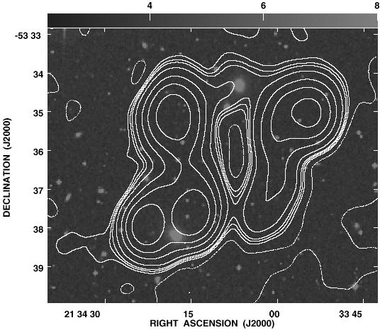
Recently an unusual exception has been discovered: a disk galaxy hosting a large double-lobed radio source (Figure 2), almost perpendicular to its disk, and several times the optical galaxy size ([Ledlow et al. (1998)]).
|
Figure 2.
VLA contours at 1.5GHz of B0313-192 in the galaxy cluster
A428, overlaid on an R-band image. The radio source extends
|
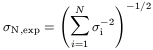
An approach to semi-automated optical identification of radio sources using the Digitized Sky Survey is described in [Haigh et al. (1997)]. However, Figure 3 shows one of the more complicated examples from this paper. Note also that the concentric contours near the centre of the radio source encircle a local minimum, and not a maximum. To avoid such ambiguities some software packages (e.g. ``NOD2'', [Haslam (1974)]) produce arrowed contours indicating the direction of the local gradient in the map.
|
Figure 3. 408MHz contours from the Molonglo Observatory Synthesis Telescope (MOST) of a complex radio source in the galaxy cluster A3785, overlaid on the Digitized Sky Survey. The source is a superposition of two wide-angle tailed (WAT) sources associated with the two brightest galaxies in the image, as confirmed by higher-resolution ATCA maps (from Haigh et al. 1997, ctsy. A. Haigh) |
Morphological considerations can sometimes lead to interesting misinterpretations. A linear feature detected in a Galactic plane survey with the Effelsberg 100-m dish had been interpreted as probably being an optically obscured radio galaxy behind our Galaxy ([Seiradakis et al. (1985)]). It was not until five years later ([Landecker et al. (1990)]) that interferometer maps taken with the Dominion Radio Astrophysical Observatory (DRAO; www.drao.nrc.ca) revealed that the linear feature was merely the straighter part of the shell of a weak and extended supernova remnant (G 65.1+0.6).
One of the most difficult classes of source to identify optically are the so-called ``relic'' radio sources, typically occurring in clusters of galaxies, with a very steep radio continuum spectrum, and without clear traces of association with any optical galaxy in their host cluster. Examples can be found in [Giovannini et al. (1991)], [Feretti et al. (1997)], or [Röttgering et al. (1997)]. See astro-ph/9805367 for the latest speculation on their origin.
Generally source catalogues are produced only for detections
above the 3-5 level. However,
[Lewis (1995)] and
[Moran et
al. (1996)]
have shown that a cross-identification
between catalogues at different wavelengths allows the
``detection'' of real sources even down to the
2 level.