


The modern physical description of the universe as a whole can be traced back to Einstein, who argued theoretically for the so-called ``cosmological principle'': that the distribution of matter and energy must be homogeneous and isotropic on the largest scales. Today isotropy is well established (see the review by Wu, Lahav, & Rees 1999) for the distribution of faint radio sources, optically-selected galaxies, the X-ray background, and most importantly the cosmic microwave background (henceforth, CMB; see, e.g., Bennett et al. 1996). The constraints on homogeneity are less strict, but a cosmological model in which the universe is isotropic but significantly inhomogeneous in spherical shells around our special location is also excluded (Goodman 1995).
In General Relativity, the metric for a space which is spatially homogeneous and isotropic is the Robertson-Walker metric, which can be written in the form
| (2) |
where
a(t) is the cosmic scale factor which describes expansion
in time,
and (R,  ,
,
 ) are spherical comoving
coordinates. The constant
k determines the geometry of the metric; it is positive in a closed
universe, zero in a flat universe, and negative in an open
universe. Observers at rest remain at rest, at fixed
(R, ,
), with their physical
separation increasing with time
in proportion to a(t). A given observer sees a nearby observer at
physical distance D receding at the Hubble velocity
H(t)D, where
the Hubble constant at time t is
H(t) = d ln a(t) / dt. Light
emitted by
a source at time t is observed at t = 0 with a redshift
z = 1 / a(t) - 1, where we set
a(t = 0)
) are spherical comoving
coordinates. The constant
k determines the geometry of the metric; it is positive in a closed
universe, zero in a flat universe, and negative in an open
universe. Observers at rest remain at rest, at fixed
(R, ,
), with their physical
separation increasing with time
in proportion to a(t). A given observer sees a nearby observer at
physical distance D receding at the Hubble velocity
H(t)D, where
the Hubble constant at time t is
H(t) = d ln a(t) / dt. Light
emitted by
a source at time t is observed at t = 0 with a redshift
z = 1 / a(t) - 1, where we set
a(t = 0)  1.
1.
The Einstein field equations of General Relativity yield the Friedmann equation (e.g., Weinberg 1972; Kolb & Turner 1990)
| (3) |
which relates the
expansion of the universe to its matter-energy content. For each
component of the energy density
 , with an equation
of state p =
p(),
the density
varies with a(t) according to the equation of energy conservation
, with an equation
of state p =
p(),
the density
varies with a(t) according to the equation of energy conservation
| (4) |
With the critical density
| (5) |
defined as the density needed for k = 0, we define the ratio of the total density to the critical density as

| (6) |
With  m,
m,
 , and
r denoting
the present contributions to
from matter (including cold dark
matter as well as a contribution
b from baryons), vacuum
density (cosmological constant), and radiation, respectively, the
Friedmann equation becomes
, and
r denoting
the present contributions to
from matter (including cold dark
matter as well as a contribution
b from baryons), vacuum
density (cosmological constant), and radiation, respectively, the
Friedmann equation becomes
| (7) |
where we define H0 and
0 =
m +
+
r to be the present
values of H and ,
respectively, and we let
| (8) |
In the particularly simple Einstein-de Sitter model
(m = 1,
=
r =
k = 0), the scale
factor varies as a(t)
 t2/3. Even models with non-zero
or
k approach the
Einstein-de Sitter behavior at high redshifts, i.e., when
t2/3. Even models with non-zero
or
k approach the
Einstein-de Sitter behavior at high redshifts, i.e., when

| (9) |
(as long as r can
be neglected). The Friedmann equation implies
that models with k
= 0 converge to the Einstein-de Sitter limit
faster than do open models. E.g., for
m = 0.3 and
= 0.7 equation (9)
corresponds to the
condition z >> 1.3, which is easily satisfied by the reionization
redshift. In this high-z regime, H(t)
 2 / (3t), and the age
of the universe is
2 / (3t), and the age
of the universe is
| (10) |
where in the last expression we assumed our standard cosmological parameters (see the end of Section 1).
In the standard hot Big Bang model, the universe is initially hot and the energy density is dominated by radiation. The transition to matter domination occurs at z ~ 104, but the universe remains hot enough that the gas is ionized, and electron-photon scattering effectively couples the matter and radiation. At z ~ 1200 the temperature drops below ~ 3300 K and protons and electrons recombine to form neutral hydrogen. The photons then decouple and travel freely until the present, when they are observed as the CMB.
2.2. Linear Gravitational Growth
Observations of the CMB (e.g., Bennett et al. 1996) show that the universe at recombination was extremely uniform, but with spatial fluctuations in the energy density and gravitational potential of roughly one part in 105. Such small fluctuations, generated in the early universe, grow over time due to gravitational instability, and eventually lead to the formation of galaxies and the large-scale structure observed in the present universe.
As in the previous section, we distinguish between fixed and comoving
coordinates. Using vector notation, the fixed coordinate r
corresponds to a comoving position x = r / a. In a
homogeneous universe with density
, we describe the
cosmological expansion
in terms of an ideal pressure-less fluid of particles each of which is
at fixed x, expanding with the Hubble flow
v = H(t)r where
v = dr / dt. Onto this uniform expansion we
impose small perturbations, given by a relative density perturbation
| (11) |
where the mean
fluid density is
 , with a
corresponding peculiar velocity
u v -
Hr. Then the fluid is described by the
continuity and Euler equations in comoving coordinates
(Peebles 1980,
1993):
, with a
corresponding peculiar velocity
u v -
Hr. Then the fluid is described by the
continuity and Euler equations in comoving coordinates
(Peebles 1980,
1993):
| (12) | 
| (13) |
The potential is
given by the Poisson equation, in terms of the density perturbation:
| (14) |
This fluid description is valid for describing the evolution of collisionless cold dark matter particles until different particle streams cross. This ``shell-crossing'' typically occurs only after perturbations have grown to become non-linear, and at that point the individual particle trajectories must in general be followed. Similarly, baryons can be described as a pressure-less fluid as long as their temperature is negligibly small, but non-linear collapse leads to the formation of shocks in the gas.
For small perturbations  <<
1, the fluid equations can be linearized and combined to yield
<<
1, the fluid equations can be linearized and combined to yield
| (15) |
This linear equation has in general two independent solutions, only one of which grows with time. Starting with random initial conditions, this ``growing mode'' comes to dominate the density evolution. Thus, until it becomes non-linear, the density perturbation maintains its shape in comoving coordinates and grows in proportion to a growth factor D(t). The growth factor is in general given by (Peebles 1980)
| (16) |
where we neglect r
when considering halos forming at
z << 104. In the Einstein-de Sitter model (or, at high
redshift, in other
models as well) the growth factor is simply proportional to a(t).
The spatial form of the initial density fluctuations can be described in Fourier space, in terms of Fourier components
| (17) |
Here we use the
comoving wavevector k, whose magnitude k is the comoving
wavenumber which is equal to 2 divided by the wavelength. The
Fourier description is particularly simple for fluctuations generated
by inflation (e.g.,
Kolb & Turner 1990).
Inflation generates
perturbations given by a Gaussian random field, in which different
k-modes are statistically independent, each with a random
phase. The statistical properties of the fluctuations are determined
by the variance of the different k-modes, and the variance is
described in terms of the power spectrum P(k) as follows:
divided by the wavelength. The
Fourier description is particularly simple for fluctuations generated
by inflation (e.g.,
Kolb & Turner 1990).
Inflation generates
perturbations given by a Gaussian random field, in which different
k-modes are statistically independent, each with a random
phase. The statistical properties of the fluctuations are determined
by the variance of the different k-modes, and the variance is
described in terms of the power spectrum P(k) as follows:
| (18) |
where (3) is the
three-dimensional Dirac delta function.
In standard models, inflation produces a primordial power-law spectrum
P(k)
kn with n ~ 1. Perturbation growth in the
radiation-dominated and then matter-dominated universe results in a
modified final power spectrum, characterized by a turnover at a scale
of order the horizon cH-1 at matter-radiation equality, and a
small-scale asymptotic shape of
P(k)
kn - 4. On large
scales the power spectrum evolves in proportion to the square of the
growth factor, and this simple evolution is termed linear
evolution. On small scales, the power spectrum changes shape due to
the additional non-linear gravitational growth of perturbations,
yielding the full, non-linear power spectrum. The overall amplitude of
the power spectrum is not specified by current models of inflation,
and it is usually set observationally using the CMB temperature
fluctuations or local measures of large-scale structure.
Since density fluctuations may exist on all scales, in order to
determine the formation of objects of a given size or mass it is
useful to consider the statistical distribution of the smoothed
density field. Using a window function W(y) normalized so that
 d3y W(y) = 1, the smoothed
density perturbation field,
d3y
(x +
y)W(y), itself follows a Gaussian
distribution with zero mean. For the particular choice of a spherical
top-hat, in which W = 1 in a sphere of radius R and is
zero outside,
the smoothed perturbation field measures the fluctuations in the mass
in spheres of radius R. The normalization of the present power
spectrum is often specified by the value of
d3y W(y) = 1, the smoothed
density perturbation field,
d3y
(x +
y)W(y), itself follows a Gaussian
distribution with zero mean. For the particular choice of a spherical
top-hat, in which W = 1 in a sphere of radius R and is
zero outside,
the smoothed perturbation field measures the fluctuations in the mass
in spheres of radius R. The normalization of the present power
spectrum is often specified by the value of
 8
(R =
8h-1Mpc). For the top-hat, the smoothed
perturbation field is denoted
R or
M, where the mass
M is related to the comoving radius R by
M = 4
m
R3 / 3,
in terms of the current mean density of matter
m. The
variance
< M >2 is
8
(R =
8h-1Mpc). For the top-hat, the smoothed
perturbation field is denoted
R or
M, where the mass
M is related to the comoving radius R by
M = 4
m
R3 / 3,
in terms of the current mean density of matter
m. The
variance
< M >2 is
| (19) |
where j1(x) = (sin x - x cos
x) / x2. The function
(M) plays a crucial role in
estimates of the abundance of collapsed objects, as described below.
2.3. Formation of Nonlinear Objects
The small density fluctuations evidenced in the CMB grow over time as
described in the previous subsection, until the perturbation
becomes of order unity, and the full non-linear gravitational problem
must be considered. The dynamical collapse of a dark matter halo can
be solved analytically only in cases of particular symmetry. If we
consider a region which is much smaller than the horizon
cH-1,
then the formation of a halo can be formulated as a problem in
Newtonian gravity, in some cases with minor corrections coming from
General Relativity. The simplest case is that of spherical symmetry,
with an initial (t = ti <<
t0) top-hat of uniform overdensity
i inside a sphere
of radius R. Although this model is
restricted in its direct applicability, the results of spherical
collapse have turned out to be surprisingly useful in understanding
the properties and distribution of halos in models based on cold dark
matter.
The collapse of a spherical top-hat is described by the Newtonian equation (with a correction for the cosmological constant)
| (20) |
where r is
the radius in a fixed (not comoving) coordinate frame,
H0 is the
present Hubble constant, M is the total mass enclosed within radius
r, and the initial velocity field is given by the Hubble flow
dr / dt = H(t)r. The enclosed
grows initially as
L =
i
D(t) / D(ti), in accordance with
linear theory, but
eventually grows above
L. If the mass shell at
radius r is bound (i.e., if its total Newtonian energy is negative)
then it reaches a radius of maximum expansion and subsequently
collapses. At the moment when the top-hat collapses to a point, the
overdensity predicted by linear theory is
(Peebles 1980)
L = 1.686 in the
Einstein-de Sitter model, with only a weak dependence on
m and
. Thus a top-hat
collapses at redshift z if its
linear overdensity extrapolated to the present day (also termed the
critical density of collapse) is
| (21) |
where we set D(z = 0) = 1.
Even a slight violation of the exact symmetry of the initial
perturbation can prevent the top-hat from collapsing to a
point. Instead, the halo reaches a state of virial equilibrium by
violent relaxation (phase mixing). Using the virial theorem U = -
2K to
relate the potential energy U to the kinetic energy K in
the final
state, the final overdensity relative to the critical density at the
collapse redshift is
 c =
182
c =
182
 178 in the Einstein-de
Sitter model, modified in a universe with
m +
= 1 to the fitting formula
(Bryan & Norman 1998)
178 in the Einstein-de
Sitter model, modified in a universe with
m +
= 1 to the fitting formula
(Bryan & Norman 1998)
| (22) |
where d
mz - 1
is evaluated at the collapse redshift, so that
| (23) |
A halo of mass M collapsing at redshift z thus has a (physical) virial radius
| (24) |
and a corresponding circular velocity,

| (25) |
In these expressions we have assumed a present Hubble constant written in the form H0 = 100 h km s-1Mpc-1. We may also define a virial temperature

| (26) |
where µ is the mean molecular weight and mp is the proton mass. Note that the value of µ depends on the ionization fraction of the gas; µ = 0.59 for a fully ionized primordial gas, µ = 0.61 for a gas with ionized hydrogen but only singly-ionized helium, and µ = 1.22 for neutral primordial gas. The binding energy of the halo is approximately (3)

| (27) |
Note that the binding energy of the baryons
is smaller by a factor equal to the baryon fraction
b /
m.
Although spherical collapse captures some of the physics governing the formation of halos, structure formation in cold dark matter models proceeds hierarchically. At early times, most of the dark matter is in low-mass halos, and these halos continuously accrete and merge to form high-mass halos. Numerical simulations of hierarchical halo formation indicate a roughly universal spherically-averaged density profile for the resulting halos (Navarro, Frenk, & White 1997, hereafter NFW), though with considerable scatter among different halos (e.g., Bullock et al. 2001). The NFW profile has the form
| (28) |
where x = r / rvir, and the
characteristic density
c is related to
the concentration parameter cN by
| (29) |
The concentration parameter itself depends on the halo mass M, at a given redshift z. We note that the dense, cuspy halo profile predicted by CDM models is not apparent in the mass distribution derived from measurements of the rotation curves of dwarf galaxies (e.g., de Blok & McGaugh 1997; Salucci & Burkert 2000), although observational and modeling uncertainties may preclude a firm conclusion at present (van den Bosch et al. 2000; Swaters, Madore, & Trewhella 2000).
2.4. The Abundance of Dark Matter Halos
In addition to characterizing the properties of individual halos, a critical prediction of any theory of structure formation is the abundance of halos, i.e., the number density of halos as a function of mass, at any redshift. This prediction is an important step toward inferring the abundances of galaxies and galaxy clusters. While the number density of halos can be measured for particular cosmologies in numerical simulations, an analytic model helps us gain physical understanding and can be used to explore the dependence of abundances on all the cosmological parameters.
A simple analytic model which successfully matches most of the
numerical simulations was developed by
Press & Schechter
(1974).
The model is based on the ideas of a Gaussian random field of density
perturbations, linear gravitational growth, and spherical collapse. To
determine the abundance of halos at a redshift z, we use
M,
the density field smoothed on a mass scale M, as defined in
Section 2.2. Although the model is based on the
initial conditions,
it is usually expressed in terms of redshift-zero quantities. Thus, we
use the linearly-extrapolated density field, i.e., the initial density
field at high redshift extrapolated to the present by simple
multiplication by the relative growth factor (see
Section 2.2). Similarly, in this section the `present
power spectrum'
refers to the initial power spectrum, linearly-extrapolated to the
present without including non-linear evolution. Since
M is
distributed as a Gaussian variable with zero mean and standard
deviation (M) [which
depends only on the present power
spectrum, see equation (19)], the probability that
M is greater than
some equals
| (30) |
The fundamental ansatz is to identify this
probability with the fraction of dark matter particles which are part
of collapsed halos of mass greater than M, at redshift z. There
are two additional ingredients: First, the value used for
is
crit(z)
given in equation (21), which is the
critical density of collapse found for a spherical top-hat
(extrapolated to the present since
(M) is calculated using the
present power spectrum); and second, the fraction of dark matter in
halos above M is multiplied by an additional factor of 2 in order to
ensure that every particle ends up as part of some halo with
M > 0. Thus, the final formula for the mass fraction in halos above
M at redshift z is
| (31) |
This ad-hoc factor of 2 is necessary, since otherwise only positive
fluctuations of M
would be included.
Bond et al. (1991)
found an alternate derivation of this correction factor, using a
different ansatz. In their derivation, the factor of 2 has a more
satisfactory origin, namely the so-called ``cloud-in-cloud'' problem:
For a given mass M, even if
M is smaller than
crit(z),
it is possible that the corresponding region lies inside a
region of some larger mass ML > M, with
ML
> crit(z).
In this case the original region should be counted as
belonging to a halo of mass ML. Thus, the fraction of
particles
which are part of collapsed halos of mass greater than M is larger
than the expression given in equation (30). Bond et al. showed
that, under certain assumptions, the additional contribution results
precisely in a factor of 2 correction.
Differentiating the fraction of dark matter in halos above M yields the mass distribution. Letting dn be the comoving number density of halos of mass between M and M + dM, we have
| (32) |
where  c =
crit(z) /
(M) is the number of
standard deviations which the critical
collapse overdensity represents on mass scale M. Thus, the abundance
of halos depends on the two functions
(M) and
crit(z),
each of which depends on the energy content of the
universe and the values of the other cosmological parameters. We
illustrate the abundance of halos for our standard choice of the
CDM model with
m = 0.3 (see the end of
Section 1).
c =
crit(z) /
(M) is the number of
standard deviations which the critical
collapse overdensity represents on mass scale M. Thus, the abundance
of halos depends on the two functions
(M) and
crit(z),
each of which depends on the energy content of the
universe and the values of the other cosmological parameters. We
illustrate the abundance of halos for our standard choice of the
CDM model with
m = 0.3 (see the end of
Section 1).
Figure 5 shows
(M) and
crit(z), with
the input power spectrum computed from Eisenstein & Hu (1999). The
solid line is (M) for
the cold dark matter model with the
parameters specified above. The horizontal dotted lines show the value
of crit(z)
at z = 0, 2, 5, 10, 20 and 30, as indicated
in the figure. From the intersection of these horizontal lines with
the solid line we infer, e.g., that at z = 5 a 1 -
fluctuation
on a mass scale of 2 × 10⁷
M will
collapse. On the other hand, at z = 5 collapsing halos require a 2 -
fluctuation on a
mass scale of 3 × 10¹⁰
M, since
(M) on this
mass scale equals about half of
crit(z =
5). Since at
each redshift a fixed fraction (31.7%) of the total dark matter
mass lies in halos above the 1 -
mass,
Figure 5 shows
that most of the mass is in small halos at high redshift, but it
continuously shifts toward higher characteristic halo masses at lower
redshift. Note also that
(M) flattens at low
masses because of the changing shape of the power spectrum. Since
->
will
collapse. On the other hand, at z = 5 collapsing halos require a 2 -
fluctuation on a
mass scale of 3 × 10¹⁰
M, since
(M) on this
mass scale equals about half of
crit(z =
5). Since at
each redshift a fixed fraction (31.7%) of the total dark matter
mass lies in halos above the 1 -
mass,
Figure 5 shows
that most of the mass is in small halos at high redshift, but it
continuously shifts toward higher characteristic halo masses at lower
redshift. Note also that
(M) flattens at low
masses because of the changing shape of the power spectrum. Since
->
 as
M -> 0, in the cold dark matter model all the
dark matter is tied up in halos at all redshifts, if sufficiently
low-mass halos are considered.
as
M -> 0, in the cold dark matter model all the
dark matter is tied up in halos at all redshifts, if sufficiently
low-mass halos are considered.

|
Figure 5.
Mass fluctuations and collapse thresholds in cold dark matter
models. The horizontal dotted lines show the value of the extrapolated
collapse overdensity
|
Also shown in Figure 5 is the effect of cutting off the
power spectrum on small scales. The short-dashed curve corresponds to
the case where the power spectrum is set to zero above a comoving
wavenumber k = 10 Mpc-1, which corresponds to a mass
M = 1.7 × 10⁸
M. The
long-dashed curve corresponds to a
more radical cutoff above k = 1 Mpc-1, or below
M = 1.7 × 10¹¹
M. A cutoff
severely reduces the
abundance of low-mass halos, and the finite value of
(M = 0)
implies that at all redshifts some fraction of the dark matter does
not fall into halos. At high redshifts where
crit(z) >>
(M = 0), all halos
are rare and only a small fraction of the dark
matter lies in halos. In particular, this can affect the abundance of
halos at the time of reionization, and thus the observed limits on
reionization constrain scenarios which include a small-scale cutoff in
the power spectrum
(Barkana, Haiman, &
Ostriker 2000).
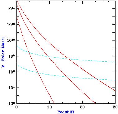
In Figures 6 - 9 we show
explicitly the properties of collapsing halos which represent 1 -
, 2 -
,
and 3 - fluctuations
(corresponding in all cases to the curves
in order from bottom to top), as a function of redshift. No cutoff is
applied to the power spectrum. Figure 6 shows
the halo mass, Figure 7 the virial radius,
Figure 8 the virial
temperature (with µ in equation (26) set equal to 0.6,
although low temperature halos contain neutral gas) as well as
circular velocity, and Figure 9 shows the total binding
energy of these halos. In Figures 6 and
8, the
dashed curves indicate the minimum virial temperature required for
efficient cooling (see Section 3.3) with
primordial atomic species
only (upper curve) or with the addition of molecular hydrogen (lower
curve). Figure 9 shows the binding energy of
dark matter halos. The binding energy of the baryons is a factor
~ b /
m ~ 15% smaller,
if they follow the dark
matter. Except for this constant factor, the figure shows the minimum
amount of energy that needs to be deposited into the gas in order to
unbind it from the potential well of the dark matter. For example, the
hydrodynamic energy released by a single supernovae,
~ 1051 erg, is sufficient to unbind the gas in all 1 -
halos at z  5
and in all 2 - halos at
z 12.
5
and in all 2 - halos at
z 12.
|
Figure 6.
Characteristic properties of collapsing halos: Halo mass.
The solid curves show the mass of collapsing halos which correspond to
1 - |

|
Figure 7.
Characteristic properties of collapsing halos: Halo virial
radius. The curves show the virial radius of collapsing halos which
correspond to 1 - |

|
Figure 8.
Characteristic properties of collapsing halos: Halo virial
temperature and circular velocity. The solid curves show the virial
temperature (or, equivalently, the circular velocity) of collapsing
halos which correspond to 1 - |

|
Figure 9.
Characteristic properties of collapsing halos: Halo binding
energy. The curves show the total binding energy of collapsing halos
which correspond to 1 - |
At z = 5, the halo masses which correspond to 1 -
, 2 -
,
and 3 - fluctuations are
1.8 × 10⁷
M,
3.0 × 10¹⁰
M, and
7.0 × 10¹¹
M,
respectively. The corresponding virial temperatures are
2.0 × 10³ K,
2.8 × 10⁵ K, and 2.3 × 10⁶ K. The
equivalent circular velocities are 7.5
km s-1, 88 km s-1, and
250 kmI>s-1. At z = 10, the 1 -
, 2 -
, and 3 -
fluctuations correspond to halo masses of 1.3 × 10³
M,
5.7 × 10⁷
M, and
4.8 × 10⁹
M,
respectively. The corresponding virial temperatures are 6.2 K,
7.9 × 10³ K, and
1.5 × 10⁵ K. The equivalent circular
velocities are 0.41 km s-1, 15
km s-1, and 65
km s-1. Atomic cooling is efficient at
Tvir
104 K, or
a circular velocity Vc
17 km
s-1. This
corresponds to a 1.2 -
fluctuation and a halo mass of
2.1 × 10⁸
M at
z = 5, and a 2.1 -
fluctuation and a halo mass of 8.3 × 10⁷
M at
z = 10. Molecular hydrogen
provides efficient cooling down to Tvir ~ 300 K, or a
circular velocity Vc ~ 2.0 km
s-1. This corresponds
to a 0.76 - fluctuation and
a halo mass of 3.5 × 10⁵
M at
z = 5, and a 1.3 -
fluctuation and a halo mass of 1.4 × 10⁵
M at z = 10.
In Figure 10 we show the halo mass function dn / d ln(M) at several different redshifts: z = 0 (solid curve), z = 5 (dotted curve), z = 10 (short-dashed curve), z = 20 (long-dashed curve), and z = 30 (dot-dashed curve). Note that the mass function does not decrease monotonically with redshift at all masses. At the lowest masses, the abundance of halos is higher at z > 0 than at z = 0.

|
Figure 10. Halo mass function at several redshifts: z = 0 (solid curve), z = 5 (dotted curve), z = 10 (short-dashed curve), z = 20 (long-dashed curve), and z = 30 (dot-dashed curve). |
3 The coefficient of 1/2 in
equation (27) would be exact for a singular isothermal
sphere, (r)
1 / r2.
Back.