3. LUMINOSITY FUNCTIONS

To address the question of how much mass different galaxies contribute to the total, we begin by examining their luminosities, which are more directly observable. The emission from a set of galaxies in a particular waveband or in a spectral line can be characterized by a luminosity function . This is a distribution function (essentially a histogram) of the number of galaxies in each range of luminosity. Luminosity functions have some generally common characteristics that we will examine in this section, and we will begin to look at how a luminosity function is translated into a mass function - which is our ultimate goal.

The function is often written as a density so that integrating over all luminosities (L)dL gives the total number of galaxies per some volume unit like 1 Mpc³. Since dL gives the total number of galaxies of each luminosity, it can be multiplied by other galaxy properties and integrated to derive population totals (or totals within narrower luminosity ranges) for other properties. For example, the total luminosity of a population is:

(1)

In principle, if we know the relationship between mass and luminosity we can integrate

(2)

to determine the total mass. This however assumes some simple relationship between mass and luminosity, which may not be realistic as we shall discuss further below.

Classically, is determined in a well-studied region where the galaxy distances are known and deep integrations have generated quite complete samples. This has usually confined such studies to nearby galaxy clusters, which is a point to keep in mind in case there are biases in the galaxy properties in such high density regions.

One of the features of galaxy luminosity functions that appears to be true at most wavelengths is that the number counts grow larger at fainter luminosities like the luminosity to some negative power. This power law behavior, (L) L where < 0, is a common sort of distribution in nature, describing the size distribution of asteroids and turbulence for example.

The power law behavior of appears to persist over several orders of magnitude in galaxy luminosity. At very high luminosities the number counts of galaxies drop off much more rapidly than the power law, and at very low luminosities the definition of a galaxy must break down as the luminosity approaches the range of globular clusters. The faint end is not very well observed though, so this low-luminosity turnover or cutoff has not been characterized.

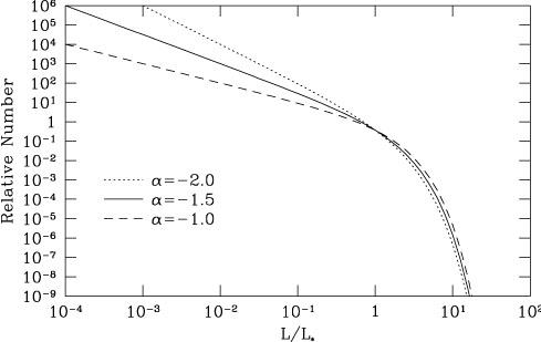
One frequently employed description of the luminosity function is that developed by Schechter (1976). The Schechter function is a power law with an exponential drop-off at high luminosities:

(3)

This function is plotted in Figure 3. The value L_* characterizes the highest luminosities before the number counts start to drop off significantly from the power law distribution. L_* is the luminosity of the most common type of bright galaxy, which are therefore some of the better known, and is approximately the luminosity of the Milky Way and M31.

Figure 3. The distribution of galaxy luminosities or masses as modeled by the Schechter luminosity function assuming different power law indices.

We can use the Schechter function to explore which galaxies contribute most to the total luminosity of galaxies. In Figure 3, the shape of the luminosity function is shown for values of the power law index from -1 to -2. The shapes of these functions do not look very different, but the resultant fraction of the luminosity contributed by different decades of luminosity is quite different, as shown in Figure 4. If the power law is shallower, the main contribution to the total luminosity is from galaxies with luminosities near L_*. However, if the power law were as steep as -2, the lowest luminosity galaxies contribute the largest fraction of light.

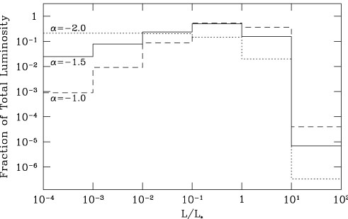
Figure 4. The total contribution to the luminosity function from different luminosity decades when assuming different power law indices in a Schechter luminosity function.

Estimates of the Schechter function generally indicate ~ -1.25. The power law appears to be even shallower than this outside of clusters, perhaps because the dwarf galaxies corresponding to the cluster dwarf elliptical populations have not been well-cataloged. (See Binggeli, Sandage, & Tammann 1988 for a review of luminosity function determinations.) Such shallow power laws would indicate that there is no major luminosity contribution from faint objects.

However, the more important question is what this relationship signifies for the total mass of galaxies. For example, low luminosity galaxies may have a larger mass-to-light ratio than brighter galaxies since their interstellar mediums are more weakly confined by their gravity and are probably less efficient at forming stars. If it were possible to characterize the mass-to-light ratio as another power law, M/L L, then the mass per luminosity interval would look like Figure 4 for a Schechter exponent of ' = + . (Note that this is not the same as the power law exponent in the mass function - the number per mass interval - which would have a distribution function obeying (M) dM = (L) dL.) If is negative as I have argued, then ' would be closer to -2 than , and low luminosity galaxies would be more significant contributors to the total mass than they are to the total luminosity.