4.3. Stress-energy tensor

The Einstein field eqs. (4.7) show that the stress-energy tensor provides the source for the metric variables. For a perfect fluid the stress-energy tensor takes the well-known form

(4.18)

where and p are the proper energy density and pressure in the fluid rest frame and u^µ = dx^µ / d (where d² - ds²) is the fluid 4-velocity. In any locally flat coordinate system, T⁰⁰ represents the energy density, T⁰ⁱ the energy flux density (which equals the momentum density Tⁱ⁰), and T^ij represents the spatial stress tensor. In locally flat coordinates in the fluid frame, T⁰⁰ = , T⁰ⁱ = 0, and T^ij = p^ij for a perfect fluid.

For an imperfect fluid such as a sum of several uncoupled components (e.g., photons, neutrinos, baryons, and cold dark matter), the stress-energy tensor must include extra terms corresponding in a weakly collisional gas to shear and bulk viscosity, thermal conduction, and other physical processes. We may write the general form as

(4.19)

Without loss of generality we can require ^µ to be traceless and flow-orthogonal: _µ^µ = 0, ^µ u = 0. In locally flat coordinates in the fluid rest frame only the spatial components ^ij are nonzero (but their trace vanishes) and the spatial stress is T^ij = p^ij + ^ij. With these restrictions on ^µ (in particular, the absence of a ⁰ⁱ term in the fluid rest frame) we implicitly define u^µ so that u^µ is the energy current 4-vector (as opposed, for example, to the particle mass times the number current 4-vector for the baryons or other conserved particles). As a result of these conditions, u^µ includes any heat conduction, p includes any bulk viscosity (the isotropic stress generated when an imperfect fluid is rapidly compressed or expanded), and ^µ (called the shear stress) includes shear viscosity. Some workers add to eq. (4.19) terms proportional to the 4-velocity, q^µ u + u^µ q, where q^µ is the energy current in the particle frame (taking u^µ to be proportional to the particle number current). Either choice is fully general, although our choice is the simplest.

We shall need to evaluate the stress-energy components in the comoving coordinate frame implied by eq. (4.11). This requires specifying the form of the 4-velocity u^µ. Therefore we must digress to discuss the 4-velocity components in a perturbed spacetime.

Consider first the case where the fluid is at rest in the comoving frame, i.e., uⁱ = 0. (This condition defines the comoving frame.) Normalization (g_µ u^µ u = - 1) then requires u⁰ = a^-1(1 - ) to first order in . Lowering the components using the full 4-metric gives u₀ = - a(1 + ) and u_i = aw_i in the weak-field approximation.

The appearance of and w_i in the components u_µ for a fluid at rest in the comoving frame may appear odd. They arise because, in our coordinates, clocks run at different rates in different places if _i 0 (the coordinate time interval d corresponds to a proper time interval a()(1 + ) d) and they also have a position-dependent offset if w_i 0 (an observer at xⁱ = constant sees the clocks at xⁱ + dxⁱ running fast by an amount w_i dxⁱ). At first these may seem like strange coordinate artifacts one should avoid (this may be a motivation for the synchronous gauge in which = w_i = 0!) but they have straightforward physical interpretations: represents the gravitational redshift and w_i represents the dragging of inertial frames. We shall see later that they also can be interpreted as giving rise to "forces," allowing us to apply Newtonian intuition in general relativity. Do not forget that in general relativity we are forced to accept coordinates whose relation to proper times and distances is complicated by spacetime curvature. Therefore, it is advantageous when we can reinterpret these effects in Newtonian terms.

We define the coordinate 3-velocity

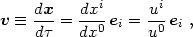(4.20)

whose components are to be raised and lowered using ^ij and _ij: v_i = _ij v^j = _ij u^j/u⁰, v² _ij vⁱv^j, w ^. v w_i vⁱ, v ^. h ^. v h_ij vⁱ v^j, etc. The 4-vector component u⁰ follows from applying the normalization condition u_µu^µ = - 1:

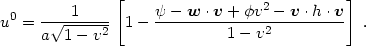(4.21)

In the absence of metric perturbations this looks like the standard result in special relativity aside from the factor a^-1 that appears because we use comoving coordinates. With metric perturbations we can no longer interpret v exactly as the proper 3-velocity because adxⁱ is not proper distance and ad is not proper time. However, the corrections are only first order in the metric perturbations.

We will assume that the mean fluid velocity is nonrelativistic so that we can neglect all terms that are quadratic in v. (This does not exclude the radiation era, since we allow individual particles to be relativistic and require only the bulk velocity to be nonrelativistic.) We will also neglect terms involving products of v and the metric perturbations. With these approximations, the 4-velocity components become

(4.22)

The apparent lack of symmetry in the spatial components arises because u_i = g_i0u⁰ + g_iju^j and g_i0 = a² w_i 0 in general.

From eq. (4.22) we can see how w_i is interpreted as a frame-dragging effect. For w_i 0 the worldline of a comoving observer (defined by the condition v_i = 0) is not normal to the hypersurfaces = constant: u_µ ^µ = aw_i ⁱ 0 for a 3-vector ⁱ. In a locally inertial frame, on the other hand, the worldline of a freely-falling observer obviously would be normal to the spatial directions. (This is true in special relativity and also in general relativity as a consequence of the equivalence principle.) By making a local Galilean transformation, dxⁱ dxⁱ + wⁱ d, we can remove w_i from the metric at a point. This transformation corresponds to choosing a locally inertial frame, called the normal frame, moving with 3-velocity - w relative to the comoving frame. In the normal frame the fluid 3-velocity is v + w.

If w_i = w_i() is independent of x, one can remove w_i everywhere from the metric by a global Galilean transformation. (Try it and see!) However, we may be interested in situations where w_i = w_i(x, ) so that different transformations are required in different places. In this case there is no global inertial frame. Spatially varying w_i corresponds to shearing and/or rotation of the comoving frame relative to the normal frame. This is called the "dragging of inertial frames." Although we can choose coordinates in which w_i = 0 everywhere, we shall see that there are advantages in not hiding the dragging of inertial frames. In general, the comoving frame is noninertial: an observer can remain at fixed xⁱ only if accelerated by nongravitational forces. The synchronous gauge is an exception in that w_i = 0 everywhere and the comoving frame is locally inertial. We shall see later that these features of synchronous gauge obscure rather than eliminate the physical dragging of inertial frames.

Now that we have all the ingredients we can finally write the stress-energy tensor components in our perturbed comoving coordinate system in terms of physical quantities:

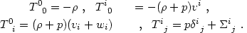(4.23)

We use mixed components in order to avoid extraneous factors of a(1 + ) and a(1 - ). Note that the traceless shear stress _jⁱ may be decomposed as in eqs. (4.13) and (4.14) into scalar, vector, and tensor parts. Similarly, the energy flux density ( + p)vⁱ may be decomposed into scalar and vector parts. (The pressure appears here, just as in special relativity, to account for the pdV work done in compressing a fluid. For a nonrelativistic fluid p << , but we shall not make this restriction.) We may already anticipate that these sources are responsible in the Einstein equations for scalar, vector, and tensor metric perturbations.

In writing the components of the stress-energy tensor we have not assumed | | << . The only approximations we make in the stress-energy tensor are to neglect (relative to unity) v² and all terms involving products of the metric perturbations with v and _jⁱ. Of course, owing to the weak-field approximation, we are also neglecting any terms that are quadratic in the metric perturbations themselves.

Before moving on to discuss the Einstein equations we should rewrite the conservation of energy-momentum, _µ T^µ = 0, in terms of our metric perturbation and fluid variables. (We use _µ to denote the full spacetime covariant derivative relative to the 4-metric g_µ. It should not be confused with the spatial gradient _i defined relative to the 3-metric _ij.) Using the approximations mentioned in the preceding paragraph, one finds

(4.24)

and

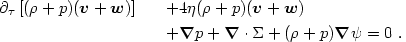(4.25)

(Deriving these gives useful practice in tensor algebra.) It is easy to interpret the various terms in these equations. The terms proportional to the expansion rate arise because we are using comoving coordinates and conformal time and have not factored out a^-3 from or p. The pressure p is present with because we let be the energy density (not the rest-mass density), which is affected by the work pressure does in compressing the fluid. Excluding these terms, the energy-conservation eq. (4.24) looks exactly like the Newtonian continuity equation aside from the change in the expansion rate from to - . This modification is easily understood by noting from eq. (4.11) that the effective isotropic expansion factor is modified by spatial curvature perturbations to become a(1 - ). The momentum-conservation eq. (4.25) similarly looks like the Newtonian version with a gravitational potential , aside from the special-relativistic effects of pressure and the addition of w to all the velocities to place them in the normal (inertial) frame.