5. FORMATION OF LARGE-SCALE STRUCTURE

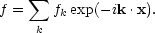
5.1. Newtonian theory for the growth of small irregularities

If the characteristic wavelength of a perturbation is much smaller than the horizon and the gravitational effects of pressure may be ignored, one can conveniently describe the evolution of irregularities within the framework of Newtonian theory (Bonnor, 1957). The justification for this comes from Birkhoff's theorem in general relativity (e.g. Weinberg, 1972, Section 11.7). Below we shall employ the fluid approximation, and the effects of matter pressure will be ignored. The equation of continuity and the Euler equation may be written,

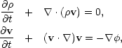(5.1a) (5.1b)

together with Poisson's equation,

(5.1c)

It proves convenient to transform from the variables (r, v) into comoving coordinates (x, u) defined by

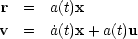(5.2a) (5.2b)

where a(t) is the cosmological scale factor and a dot denotes the derivative with respect to t. In comoving coordinates, Eqs. (5.1) read,

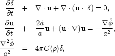(5.3a) (5.3b) (5.3c)

where is defined by (x, t) = <>(1 + ) and <> is the mean matter density. For mathematical convenience we now assume that the matter distribution is periodic in a cube of volume V_x, chosen to be large enough that any clustering on scales corresponding to V_x may be neglected, and we define the Fourier transforms of quantities such as , u, according to,

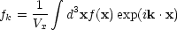(5.4a)

and the inverse transform,

(5.4b)

In terms of the Fourier transformed variables, Eqs. (5.3) take the simple form,

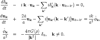(5.5a) (5.5b) (5.5c)

The terms under the summation signs represent the non-linear effects which couple modes. The main virtue of the Fourier transformed variables is that the linear theory may be applied to large wavelengths even when the matter is highly non-linear on small scales - if the mode coupling terms are small. This point will be discussed further below, but for the moment we will simply ignore the non-linear terms. In this case, the evolution of _k is given by the usual linear theory equation (e.g. Weinberg, 1972, Section 15.9)

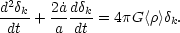(5.6)

In an Einstein-de Sitter universe, a(t) t^2/3, hence Eq. (5.6) has the power law solutions (Peebles and Dicke, 1968),

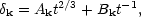(5.7a)

where A_k and B_k are fixed by specifying _k and u_k at some initial epoch t_i ,

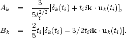(5.7b) (5.7c)

The velocity field is fixed by Eq. (5.5b),

(5.7d)

Now, in a low density universe, with present density ₀ << 1, the scale factor behaves as a t^2/3 for 1 + z >> 1 / ₀ and a t for 1 + z << 1 / ₀, hence at late times, the solutions to Eq. (5.6) take the form,

(5.8)

Hence in a low density universe, perturbations effectively stop growing at redshifts z_f 1 / ₀ - 1.

Henceforth we shall concentrate on the dominant modes in Eqs. (5.7) and (5.8) and we shall make the simplifying assumption of a power law spectrum of fluctuations,

(5.9)

where each of the A_k has a randomly assigned phase.

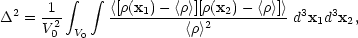
As measures of the dumpiness of the matter distribution we shall consider first the auto-correlation function (x) defined as,

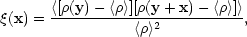(5.10)

where, the angular brackets denote an average over the volume V_x. Hence from Eq. (5.4b)

(5.11)

i.e. the auto-correlation function is just the Fourier transform of the power-spectrum |_k|². As a second measure of clustering, consider the mean square density contrast in randomly placed spheres of comoving volume V₀:

(5.12)

then by Eq. (5.10)

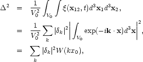(5.13)

where x₀ is the radius of the sphere of volume V₀ and,

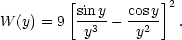Since the function W has the asymptotic behaviour, W(y) 1 for y << 1, W(y) ~ 1/y⁴ for y >> 1, Eqs. (5.13) and (5.19) yield for n < 1,

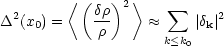(5.14)

where k₀ = 2 / x₀. If n > 1 the dominant contribution to ² comes from the side lobes of the window function W, hence ²(x₀) does not yield a good estimate of the mean square density contrast on scales x₀. Physically, this is because for a sufficiently subrandom distribution the measure ² becomes sensitive to whether clumps fall inside or outside the sharp edge of the sphere. The problem may be alleviated by weighting the integral (5.12) by factors which eliminate the side-lobes in the window function W, for example one could use Gaussians exp(- x² / 2x₀²). The mean squared density contrast may then be adequately approximated by Eq. (5.14) (Peebles and Groth (1976)).

The linear theory is expected to fail on scales x_m where <( / )²>_xm ~ 1. From Eq. (5.14),

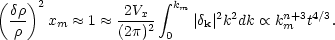(5.15)

Hence, the characteristic length scale on which perturbations are currently entering the non-linear regime of growth evolves as

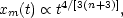(5.16)

This is an important result since it suggests a possible observational test for the index n. If n - 3, a wide range of scales will reach the non-linear regime of growth almost simultaneously, one would then expect bound structures to have almost the same internal densities independent of their size. In contrast, if n > - 3, structure on small scales will condense at an early stage when the mean density of the, Universe was much higher than it is now, one then expects that the internal densities of bound lumps would be strongly dependent on their size. These arguments will be made more quantitative in Section 5.3 below

One point of concern in the derivation of Eq. (5.16) is the justification of the validity of linear theory for _k. Indeed, Press and Schechter (1974) have argued that when the matter distribution is highly non-linear for k k_m, the mode-coupling terms in Eqs. (5.5) might become important for k << k_m invalidating the linear theory results of Eqs. (5.7) and (5.8). This problem is discussed in detail by Peebles (1974b, and 1980a, Section 28). Although it is difficult to provide a rigorous proof, Peebles' consistency argument suggests that the linear theory is valid if n < 4. If n 4, the small-scale motions of particles generate a spectrum ||² k⁴ as discussed at the end of Section 3.2. Perhaps the best test of the linear theory results come from numerical N-body experiments (Peebles and Groth, 1976; Efstathiou, 1979); these will be discussed in Section 5.3 below.