5.3. Hierarchical clustering

Under the assumption of a power-law spectrum of isothermal fluctuations at the epoch of recombination, there will be a length scale x_m ~ k_m^-1 at which <| / |²>_km ~ 1, i.e. fluctuations on scales < x_m will be non-linear. Hence after decoupling bound objects (seeds) will form of size ~ x_m and all mass scales > x_m will grow thereafter via graviational instability. Using Eqs. (5.7a), (5.8) and (5.15) we may make a crude estimate of the characteristic masses of the "seeds" that are required at recombination in order to account for the level of clustering observed today. The result is

(5.25)

typically smaller than the mass of a bright galaxy, but comparable to the Jeans mass just after recombination,

(5.26)

Hence with a power-law spectrum of fluctuations, the matter is highly non-linear on small enough scales. In order to simplify the discussion of the subsequent evolution of the system, we now make several simplifying assumptions (Davis and Peebles, 1977): (i) The initial seed masses will be considered to act as point particles with a characteristic interparticle separation ₀ which is much smaller than any length scale of interest. (ii) The seed masses account for all the mass in the universe, i.e. there does not exist a dominant hot component, such as massless (or very light m 1 eV) neutrinos. (iii) Non-gravitational processes (e.g. dissipation) will be ignored. (iv) The expansion of the universe follows that of an Einstein-de Sitter model ( = 0, = 1). One or more of these points might be in error, for example it is clear that gas dynamical processes have been important in the formation of spiral galaxies [point (iii)], also present observations suggest < 1 [point (iv)]. Possible objections to the model will be discussed in greater detail below. The main aim of the model is to predict the expected shape of the two-point correlation function (x, t). Assumptions (i)-(iv) then considerably simplify the discussion, since in this case the equations governing the evolution of (x, t) allow a similarity solution (Davis and Peebles, 1977). Assumptions (i)-(iii) guarantee that the only length scale in the problem is x_m(t) - the length scale below which perturbations are in the non-linear regime. Assumption (iv) guarantees that the expansion rate of the universe presents no characteristic timescales. If we take a snapshot of the clustering pattern at some time t₁ and compare with another snapshot taken at some later time t₂, the similarity solution states that the clustering patterns should be statistically identical apart from a change in scale x_m, i.e., we should be able to write (x, t) = (s), where the variable s is some function of x and t.

From Eqs. (5.9) and (5.11) it follows that in the linear regime << 1,

(5.27)

(Peebles, 1974). Thus, the linear evolution fixes the variable s,

(5.28)

The non-linear evolution of may then be fixed from the equation of conservation of particle pairs, (for a derivation see Peebles, 1976b),

(5.29)

Here <u₁₂> is the mean relative velocity between particle pairs. Under the similarity transformation, Eq. (5.25) becomes

(5.30)

where <u₁₂> = t^-1 <₁₂>. On small scales where >> 1, it is fairly reasonable to suppose that the clusters are bound and stable. In proper coordinates [Eq. (5.2b)] this means < v > = 0, hence

Using the assumption of small-scale stability (<> = - 2s/3) Eq. (5.30) has a solution valid for >> 1 (Davis and Peebles, 1977),

(5.31)

Similarly, an equation of conservation of triplets can be used to show that under the similarity transformation and the assumption of small scale stability the three-point correlation function (s₁₂, s₂₃, s₃₁) behaves as,

(5.32)

where the "shape" parameters u and v are held constant. The argument can can be generalized to the 4-point and higher order functions (Peebles, 1980a, Section 73). Now, the observed slope of the two-point function, = 1.8, can be matched with Eq. (5.31) by taking n = 0, and the similarity solution then accounts for the observed shapes of the three- and four-point functions.

The similarity solution of Eq. (5.31) may be understood in terms of the following simple argument (Peebles, 1974). By Eq. (5.16) the characteristic proper radius of lumps entering the non-linear regime of growth scales with time as,

(5.33)

and the mean density of the universe scales as t^-2. If the perturbations collapse and form bound and stable systems with internal densities equal to some fixed fraction of the mean background density at the time they collapsed, then Eq. (5.33) states that the internal density of bound systems will scale with proper radius as

(5.34)

as in Eq. (5.31). This leads to a picture in which the matter is hierarchically clustered, i.e. when the matter distribution is looked at with any given resolution r, the mean internal density of lumps follows the scaling relation (5.34) (cf. Section 2.4).

The observed shape of (x) approximates a power law over the range 10⁵ > 0.3, whereas the solution (5.31) only applies for >> 1; hence it is not clear whether the similarity solution is compatible with the observations in the range where 1. The behaviour of (r) in the transition region ~ 1 is a point of much current interest (e.g. Davis, Groth and Peebles, 1977) but as yet no convincing solution has emerged.

Davis and Peebles (1977) have tackled the problem using the BBGKY equations of kinetic theory. The BBGKY formalism replaces Newton's equations of motion with an infinite set of coupled equations for the reduced particle distribution functions. In order to yield a tractable problem, Davis and Peebles truncate the hierarchy by choosing a model for the three-particle distribution function which reproduces the observed relation between and [Eq. (2.28)]. Together with some subsidiary approximations, the equations are simplified to the extent that a numerical solution becomes possible. Davis and Peebles find a similarity solution for (r) which matches the observed shape quite well if n = 0 and also yields a value for the parameter Q in Eq. (2.28) in reasonable agreement with observations. Their results may be interpreted using the equation of conservation of particle pairs [Eq. (5.30)] and suggest that the velocity dispersion within a protocluster grows while it is still a small density perturbation so that when the cluster fragments out of the general expansion, it is already virialized. Thus, Davis and Peebles find that their solutions may be approximated by a two-power law model with slope given by Eq. (5.31) for > _break, and by (5.27) for < _break with _break 0.2.

In contrast, simple analytic treatments of galaxy clustering for = 1, (e.g. Gott and Rees, 1975) based on the homogeneous spherical cluster model predict _break >> 1. The reason for this discrepancy is that in the spherical cluster model, a cluster reaches maximum expansion at a density contrast / = 9² / 16 - 1 (e.g. Gunn and Gott, 1972). At this stage, the total kinetic energy T is zero, hence the cluster must collapse by a factor of 2 in order to generate enough kinetic energy to satisfy the virial theorem. Because of the collapse effect, the relative velocity between particle pairs u₂₁ exceeds the Hubble flow, Hr₂₁ in the transition region 1 and so the stability condition and Eq. (5.31) are only applicable for / 400, hence _break >> 1.

These points are illustrated by the simple analytic model shown in Figure 5.3. The two-point function is assumed to have the shape

(5.35)

which gives the correct behaviour in the non-linear and linear regimes if n = 0. The transition between the asymptotic slopes may be adjusted by varying the parameter s₁ / s₀ and the behaviour of the mean relative velocity between pairs may be computed using Eq. 5.30. In the case of curve (1), which resembles the results of Davis and Peebles, the mean relative velocity |<₁₂>| is less than (2/3)s at all pair separations. Curve (3), on the other hand, is a poor approximation to the observed shape of (r). This results in a region where |<₁₂>| > (2/3)s at around the region where (s) ~ 1. This corresponds to the collapse effect expected on the spherical cluster model. Clearly, the spherical model is likely to be a considerable oversimplification, and it may be expected that more complicated models would tend to dilute the effect. However it is difficult to judge whether Davis and Peebles have correctly modelled the clustering process or whether their results have been unduly affected by their approximations. In order to answer these questions several workers have tackled the problem using N-body simulations (Miyoshi and Kihara, 1975; Aarseth et al., 1979; Efstathiou and Eastwood, 1981).

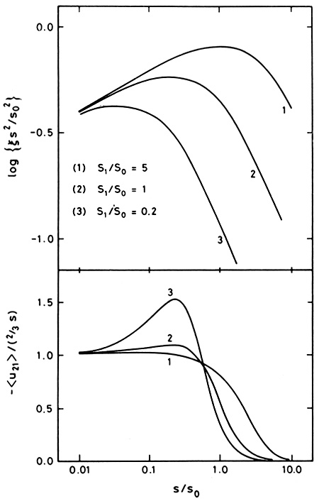Figure 5.3. The two-point correlation function and the mean relative peculiar velocity between particle pairs calculated from the model or Eq. (5.35).

The N-body approach is quite attractive, since it avoids the considerable simplifications required in the analytic approach. In a standard simulation, particles are laid down according to some prescription (e.g. a random distribution) and each particle is given a uniform Hubble velocity. The equations of motion are then integrated directly, and various statistics may be measured and compared with observations. There are, however, two important limitations in such simulations (Fall, 1978). Discrete particle effects dominate on scales less than the interparticle separation and the calculations become unreliable when clustering occurs on scales of the order of the size of the system. For N ~ 1000, this restricts the useful range of scales to less than a decade, i.e. 0.1 r 1! The large interparticle separation violates the assumptions on which the similarity solution is based, hence a direct comparison with the results of Davis and Peebles must be viewed with some caution. Nevertheless, these studies show that, to a first approximation, the two-point function develops a roughly power-law form that is somewhat steeper than is observed if Poisson initial conditions are used and = 1 (Efstathiou, Fall and Hogan, 1979). The most extensive numerical simulations to date are those of Efstathiou and Eastwood (1981). These authors use 20,000 particles which helps to increase the dynamic range in the models. Figures 5.4 and 5.5 show projections of an = 1 model with Poisson initial conditions. These models give a two-point correlation function which is steeper than the observations. The stability assumption does not apply on scales corresponding to 50. Instead, one observes a radial streaming as clusters collapse in order to generate enough kinetic energy to satisfy the virial theorem. Thus, the N-body results are similar to those illustrated by curve (3) in Figure 5.3. There is an additional important discrepancy between these N-body models and observations (Efstathiou, 1983). If the models are scaled so that (r₀) = 1 with r₀ 5h^-1 Mpc, the one-dimensional r.m.s. peculiar velocity between particle pairs of separation r₀ is <w²>^1/2 ~ 900 km sec^-1. As discussed in Section 2.4, this is much larger than the r.m.s. peculiar velocities between galaxy pairs. One way out of the problem posed by the peculiar velocities is to drop the assumption that = 1.

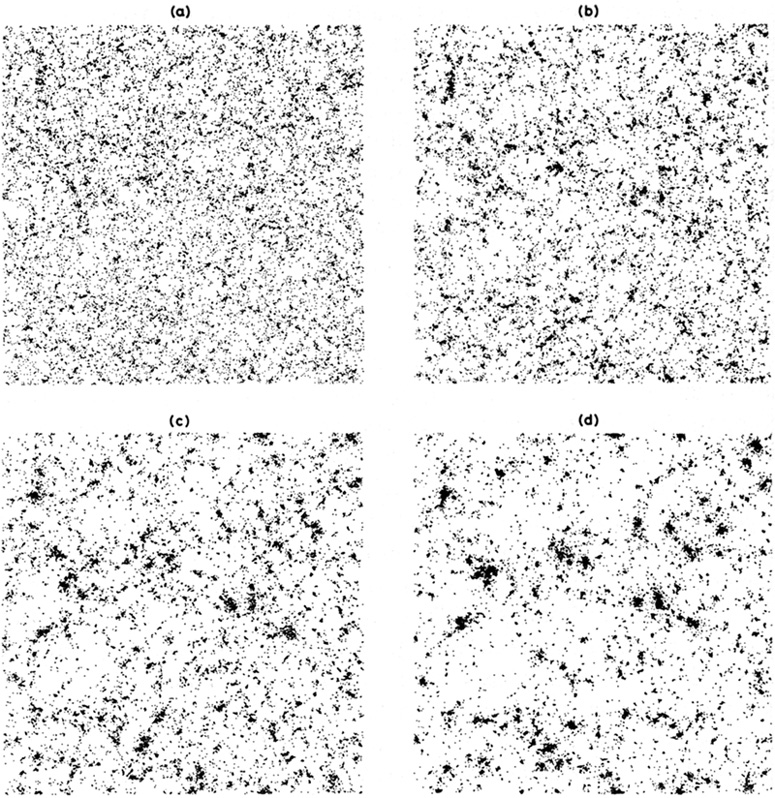Figure 5.4. Evolution of clustering in a large N-body simulation (N = 20, 000) with Poisson initial conditions and = 1. (a) Shows positions after the system has expanded by a factor of 5.1; (b) after expansion by a factor 9.8; (c) after expansion by a factor of 16.0; (d) after expansion by a factor of 28.1.

Figure 5.5. Three projections showing the final clustering pattern, after after expansion by a factor of 28.1, of the model shown in figure 5.4.

The development of in an open universe presents a much more complex problem because the conditions for a similarity solution are violated if 1. The following simple model (Peebles, 1974a) gives an indication of what might be expected. As discussed in Section 5.1 [Eq. (5.8)] the linear growth perturbations in an open Universe with present density parameter ₀ effectively ceases for redshifts z_f < 1 / ₀ - 1. Prior to this, the similarity solution should apply. Thus structures on scales such that _break will be in virial equilibrium whilst those on scales such that << _break will still be in the linear regime. For z < z_f the density contrast of bound virialized lumps will continue to increase as (1 + z)^-3 simply because of the expansion of the Universe, whilst the density contrast of structure in the linear regime will stop growing. Thus, one would expect to see a feature at _break / ₀³. Since no change in slope is observed at small scales, this has been used as an argument against gravitational instability in a low density Universe (Peebles, 1974a; Davis, Groth and Peebles, 1977). The shape of the two-point correlation function is found to be dependent on in the N-body simulations (Efstathiou, 1979; Gott, Turner and Aarseth, 1979; Fry and Peebles, 1980). In the case of Poisson initial conditions, the slope of evolves to > 2, with - 2.6 for = 0.1. Gott, Turner and Aarseth (1979) and Gott and Rees (1975) have argued that the observed clustering pattern may be consistent with a low density Universe, ₀ = 0.1, if n - 1. in this case one might expect to see a deviation from = - 1.8 on small scales, if bound virialized clumps obey the scaling law of Eq. (5.31). It may be that relaxation (White and Negroponte, 1982), or gas dynamical effects modify this prediction on small scales. There may still be a problem since the model does not predict the sharp change in slope at 0.2 which appears to be observed in the analysis of the Lick catalogue (Groth and Peebles, 1977, Section 2.4).

The N-body models also make predictions on the shape of the three-point correlation function and the parameter Q. It turns out that Eq. (2.28) is quite well obeyed and Q 1 independent of initial conditions and the value of Q.

An ingenious alternative to the standard N-body approach has been devised by Fry and Peebles (1980) and preliminary results agree qualitatively with the results described above.