3.1. Large-scale structure

Figure 1 illustrates the spatial distribution of dark matter at the present day, in a series of simulations covering a large range of scales. Each panel is a thin slice of the cubical simulation volume and shows the slightly smoothed density field defined by the dark matter particles. In all cases, the simulations pertain to the "CDM" cosmology, a flat cold dark matter model in which _dm = 0.3, = 0.7 and h = 0.7. The top-left panel illustrates the Hubble volume simulation: on these large scales, the distribution is very smooth. To reveal more interesting structure, the top right panel displays the dark matter distribution in a slice from a volume approximately 2000 times smaller. At this resolution, the characteristic filamentary appearance of the dark matter distribution is clearly visible. In the bottom-right panel, we zoom again, this time by a factor of 5.7 in volume. We can now see individual galactic-size halos which preferentially occur along the filaments, at the intersection of which large halos form that will host galaxy clusters. Finally, the bottom-left panel zooms into an individual galactic-size halo. This shows a large number of small substructures that survive the collapse of the halo and make up about 10% of the total mass (Klypin et al. 1999, Moore et al. 1999)

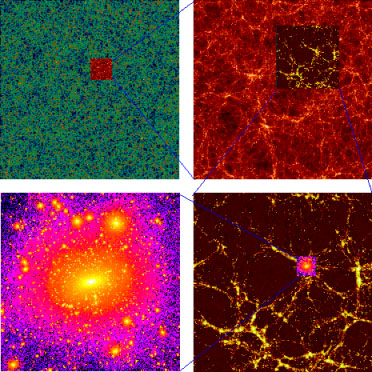Figure 1. Slices through 4 different simulations of the dark matter in the "CDM" cosmology. Denoting the number of particles in each simulation by N, the length of the simulation cube by L, the thickness of the slice by t, and the particle mass by mp, the characteristics of each panel are as follows. Top-left (the Hubble volume simulation, Evrard et al. 2002): N = 109, L = 3000 h-1 Mpc, t = 30 h-1 Mpc, mp = 2.2 × 1012 h-1 M. Top-right (Jenkins et al. 1998): N = 16.8 × 106, L = 250 h-1 Mpc, t = 25 h-1 Mpc, mp = 6.9 × 1010 h-1 M. Bottom-right (Jenkins et al. 1998): N = 16.8 × 106, L = 140 h-1 Mpc, t = 14 h-1 Mpc, mp = 1.4 × 1010 h-1 M. Bottom-left (Navarro et al. 2002): N = 7×106, L = 0.5 h-1 Mpc, t = 1 h-1 Mpc, mp = 6.5 × 105 h-1 M.

For simulations like the ones illustrated in Figure 1, it is possible to characterize the statistical properties of the dark matter distribution with very high accuracy. For example, Figure 2 shows the 2-point correlation function, (r), of the dark matter (a measure of its clustering strength) in the simulation depicted in the top-right of Figure 1 (Jenkins et al. 1998). The statistical error bars in this estimate are actually smaller than the thickness of the line. Similarly, higher order clustering statistics, topological measures, the mass function and clustering of dark matter halos and the time evolution of these quantities can all be determined very precisely from these simulations (e.g. Jenkins et al. 2001, Evrard et al. 2002). In a sense, the problem of the distribution of dark matter in the CDM model can be regarded as largely solved ⁽⁴⁾.

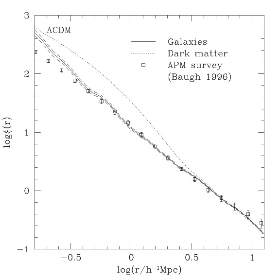Figure 2. Two-point correlation functions. The dotted line shows the dark matter dm(r) (Jenkins et al. 1998). The solid line shows the galaxy predictions of Benson et al. (2000), with Poisson errors indicated by the dashed lines. The points with errorbars show the observed galaxy gal(r) (Baugh 1996). The galaxy data are discussed in §3(b). (Adapted from Benson et al. (2001a).

In contrast to the clustering of the dark matter, the process of galaxy formation is still poorly understood. How then can dark matter simulations like those of Figure 1 be compared with observational data which, for the most part, refer to galaxies? On large scales a very important simplification applies: for Gaussian theories like CDM, it can be shown that if galaxy formation is a local process, that is, if it depends only upon local physical conditions (density, temperature, etc), then, on scales much larger than that associated with individual galaxies, the galaxies must trace the mass, i.e. on sufficiently large scales, _gal(r) _dm(r) (Coles 1993). It suffices therefore to identify a random subset of the dark matter particles in the simulation to obtain an accurate prediction for the properties of galaxy clustering on large scales. This idea (complemented on small scales by an empirical prescription in the manner described by Cole et al. 1998) has been used to construct the mock versions of a region of the APM galaxy survey and of a slice of the 2dFGRS displayed in Figures 3 and 4 which also show the real data for comparison in each case. By eye at least, it is very difficult to distinguish the mocks from the real data.

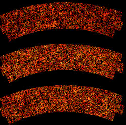Figure 3. The region of the APM projected galaxy survey from which the 2dFGRS is drawn. Only galaxies brighter than mbJ = 19.35 are plotted. The top panel is the real data and the other two panels are mock catalogues constructed from the Hubble volume simulations.

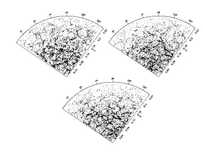Figure 4. A 1° thick slice through the 2dF galaxy redshift survey. The radial coordinate is redshift and the angular coordinate is right ascension. The top-left panel is the real data and the other two panels are mock catalogues constructed from the Hubble volume simulations.

A quantitative comparison between simulations and the real world is carried out in Figure 5. The symbols show the estimate of the power spectrum in the 2dFGRS survey (Percival et al. 2001). This is the raw power spectrum convolved with the survey window function and can be compared directly with the line showing the theoretical prediction obtained from the mock catalogues which have exactly the same window function. The agreement between the data and the CDM model is remarkably good.

Figure 5. The power spectrum of the 2dFGRS (symbols) compared with the power spectrum predicted in the CDM model (line). Both power spectra are convolved with the 2dFGRS window function. The model predictions come from dark matter simulations and assume that, on large scales, the distribution of galaxies traces the distribution of mass. (Adapted from Percival et al. 2001).

⁴ However, the innermost structure of halos like those in the bottom-left of Figure 1 is still a matter of controversy. Back.