3.6. The Future of the Loops

Loops are formed through string interactions. Their shape is arbitrary and they will (like their progenitors) move relativistically and emit gravitational radiation. This will make the loops shrink while the currents (the rotation of the current carriers), initially weak, will begin to affect the dynamics at some point. Also, the string tension will try to minimize the bending, leading to a final state of a circular and rotating ring.

Once a string loop has reached the state of a ring, it still has to be decided whether it'll become a vorton (an equilibrium configuration) or not. In [Carter, Peter & Gangui, 1997] and [Gangui, Peter & Boehm, 1998] we studied the dynamics of circular rings, including the possibility that the current be charged, so that even the contributions of the electric and magnetic fields surrounding and generated by the string were considered. This dynamics was describable in terms of a very limited number of variables, namely the ring total mass M, its rotation velocity, and the number of charges it carried. Given this, it was found that a typical loop of radius r lives in a potential (r) whose functional form depends on the Lagrangian of Eq. (45) and looks like the one shown in Figure 1.10

(74)

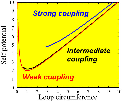
From this the force it exerts onto itself can be derived. What is represented there is the force strength, in arbitrary units of energy, exerted on the loop by itself as a function of its circumference.

Figure 1.10. Variations of the self potential with the ring's circumference = 2r and the electromagnetic self coupling (q2 in the text). The red curve stands for various values of q2 < 0.1 for which they are indistinguishable, and in the "safe" zone vorton-forming case; the minimum value of is then M, the vorton mass. for q2 = 1 is represented as the black line, where it is clear that we now are in a zone where the potential has a minimum (new value for M) but now terminates at some point. Finally the blue curve represents the potential for q2 = 10, an unrealistically large value, and this time the curve terminates even before reaching a minimum: this is a situation in which all loops with such parameters will eventually decay [Gangui, Peter & Boehm, 1998].

The loop evolution follows that of the potential: it first goes down (therefore shrinking) until it reaches the valley in the bottom of which the force vanishes, then its inertia makes it climb up again on the opposite direction where the force now tends to stop its shrinking (centrifugal barrier). At this point, two possibilities arise, depending on the initial mass available. Either this mass is not too big, less than the value of the energy where the potential ends (see the black curve), or it exceeds this energy: in the former case, the loop will bounce back and eventually oscillate around the equilibrium position at the bottom of the valley (in order to stabilize itself there, the loop will loose some energy in the form of radiation); in the latter case, it will shrink so much that its size will eventually approach the limit (its Compton length) where quantum effects will disintegrate away the ring into a burst of particles. Note the divergence for very large values of the radius r. This is nothing but the evidence that an infinite amount of energy is needed to enlarge infinitely the loop, a sort of confinement effect. In the Figure 1.10 we also see how the magnitude of the electromagnetic corrections, when strings are coupled with electric and magnetic fields, tends to reduce the number of surviving vortons: a stable configuration (red line) for a weak coupling may become unstable and collapse if its initial mass is too big for intermediate couplings (black line), or it will do so regardless of its mass in the strong coupling case (blue line).