2.10. Bounded domains and directional data

It is very often the case that the natural domain of definition of a density to be estimated is not the whole real line but an interval bounded on one or both sides. For example, both the suicide data and the Old Faithful eruption lengths are measurements of positive quantities, and so it will be preferable for many purposes to obtain density estimates for which (x) is zero for all negative x. In the case of the Old Faithful data, the problem is really of no practical importance, since there are no observations near zero, and so the lefthand boundary can simply be ignored. The suicide data are of course quite another matter. For exploratory purposes it will probably suffice to ignore the boundary condition, but for other applications, and for presentation of the data, estimates which give any weight to the negative numbers are likely to be unacceptable.

One possible way of ensuring that (x) is zero for negative x is simply to calculate the estimate for positive x ignoring the boundary conditions, and then to set (x) to zero for negative x. A drawback of this approach is that if we use a method, for example the kernel method, which usually produces estimates which are probability densities, the estimates obtained will no longer integrate to unity. To make matters worse, the contribution to ₀ (x) dx of points near zero will be much less than that of points well away from the boundary, and so, even if the estimate is rescaled to make it a probability density. the weight of the distribution near zero will be underestimated.

Some of the methods can be adapted to deal directly with data on the half-line. For example, we could use an orthogonal series estimate of the form (2.9) or (2.10) with functions which were orthonormal with respect to a weighting function a which is zero for x < 0. The maximum penalized likelihood method can be adapted simply by constraining g(x) to be zero for negative x, and using a roughness penalty functional which only depends on the behaviour of g on (0, ).

Another possible approach is to transform the data, for example by taking logarithms as in the example given in Section 2.9 above. If the density estimated from the logarithms of the data is , then standard arguments lead to

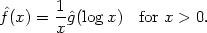
It is of course the presence of the multiplier 1/x that gives rise to the spike in Fig. 2.13; not with standing difficulties of this kind, Copas and Fryer (1980) did find estimates based on logarithmic transforms to be very useful with some other data sets.

It is possible to use other adaptations of methods originally designed for the whole real line. Suppose we augment the data by adding the reflections of all the points in the boundary, to give the set {X₁, - X₁, X₂, - X₂,...}. If a kernel estimate f^* is constructed from this data set of size 2n, then an estimate based on the original data can be given by putting

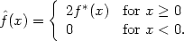
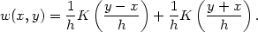
This estimate corresponds to a general weight function estimator with, for x and y > 0,

Provided the kernel is symmetric and differentiable, some easy manipulation shows that the estimate will always have zero derivative at the boundary. If the kernel is a symmetric probability density, the estimate will be a probability density. It is clear that it is not usually necessary to reflect the whole data set, since if X_i/h is sufficiently large, the reflected point - X_i/h will not be felt in the calculation of f^*(x) for x 0, and hence we need only reflect points near 0. For example, if K is the normal kernel there is no practical need to reflect points X_i > 4h.

This reflection technique can be used in conjunction with any method for density estimation on the whole line. With most methods estimates which satisfy '(0 +) = 0 will be obtained.

Another, related, technique forces (0 +) = 0 rather than '(0 +) = 0. Reflect the data as before, but give the reflected points weight -1 in the calculation of the estimate; thus the estimate is, for x 0,

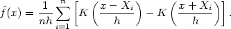
(2.16)

We shall call this technique negative reflection. Estimates constructed from (2.16) will no longer integrate to unity, and indeed the total contribution to ₀ (x)dx from points near the boundary will be small. Whether estimates of this form are useful depends on the context.

All the remarks of this section can be extended to the case where the required support of the estimator is a finite interval [a, b]. Transformation methods can be based on transformations of the form

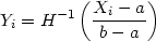
where H is any cumulative probability distribution function strictly increasing on (- , ). Generally, the estimates obtained by transformation back to the original scale will be less smoothed for points near the boundaries. The reflection methods are easily generalized. It is necessary to reflect in both boundaries and it is of course possible to use ordinary reflection in one boundary and negative reflection in the other, if the corresponding boundary conditions are required.

Another way of dealing with data on a finite interval [a, b] is to impose periodic or `wrap around' boundary conditions. Of course this approach is particularly useful if the data are actually directions or angles; the turtle data considered in Section 1.2 were of this kind. For simplicity, suppose that the interval on which the data naturally lie is [0, 1]. which can be regarded as a circle of circumference l: more general intervals are dealt with analogously. If we want to use a method like the kernel method, a possible approach is to wrap the kernel round the circle. Computationally it may be simpler to augment the data set by replicating shifted copies of it on the intervals [-1,0] and [1,2], to obtain the set

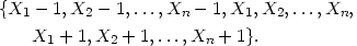
(2.17)

in principle we should continue to replicate on intervals further away from [0. 1], but that is rarely necessary in practice. Applying the kernel method or one of its variants to the augmented data set will give an estimate on [0, 1] which has the required boundary property; of course the factor 1 / n should be retained in the definition of the estimate even though the augmented data set has more than n members.

The orthogonal series estimates based on Fourier series will automatically impose periodic boundary conditions, because of the periodicity of the functions of section 2.7.