

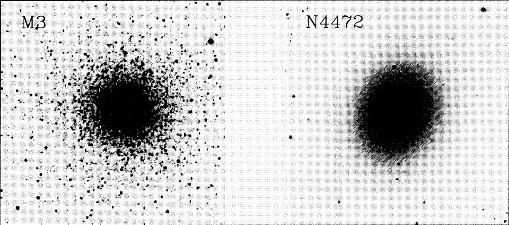
The idea behind the measurement and interpretation of surface brightness fluctuations (SBF) is simple. Figure 1 shows an image of a globular cluster (M3) and a Virgo galaxy. As far as mean surface brightness goes, the two images are nearly identical. However the globular cluster image is much more mottled.
|
Setting aside the technical difficulties, the measurement of SBF is straightforward:
 .
.
The flux that we see in a pixel is coming from a finite number N of
stars of average
flux  , and so we expect
that g = N,
and
= N1/2
, so we can solve for
this average
flux as
=
2 /
g. For example, at a radius of 1 arcmin in the bulge of M31 we
might see an I surface brightness of g = 16 mag
sec-2. Assuming we're in the limit
of no readout noise and perfect seeing so that adjacent pixels are
negligibly blurred with each other (see below how to deal with the true
situation), we might find that the
irreduceable mottling in 1" pixels gives
= 19.5 mag,
i.e. about 4 percent of the mean
brightness. We can then immediately solve for the magnitude
corresponding to as
, and so we expect
that g = N,
and
= N1/2
, so we can solve for
this average
flux as
=
2 /
g. For example, at a radius of 1 arcmin in the bulge of M31 we
might see an I surface brightness of g = 16 mag
sec-2. Assuming we're in the limit
of no readout noise and perfect seeing so that adjacent pixels are
negligibly blurred with each other (see below how to deal with the true
situation), we might find that the
irreduceable mottling in 1" pixels gives
= 19.5 mag,
i.e. about 4 percent of the mean
brightness. We can then immediately solve for the magnitude
corresponding to as
 I = 2×19.5
- 16.0 = 23.0 mag.
I = 2×19.5
- 16.0 = 23.0 mag.
There are, of course, technical difficulties. The first is that seeing
blurs pixels together, reducing the
from what it would be at
the top of the atmosphere, with only Poisson
statistics operating. Since we know accurately what the point spread
function (psf) is
from stars in the field, we can compensate for this effect and compute
what , would
be in the absence of seeing. Our method is to do this in the Fourier
domain, where
convolution by the psf becomes multiplication by the transform of the psf.
A second challenge is that there are other sources of noise. We have some detector readout noise, and there is noise from the Poisson statistics of the photons collected as well as the Poisson noise from the finite number of stars. In our method we exploit the fact that these sources of noise are not blurred by the psf and therefore have a white noise spatial power spectrum. Figure 2 illustrates schematically what the power spectrum looks like.

|
Figure 2. A schematic drawing of the SBF power spectrum. |
Galaxies can also be bumpy if the stars are correlated with each other,
either through
their own gravity, or more likely from the gravity perturbations from a
large-scale mode.
Spiral arms are an example of this, and the SBF method is not applicable
in such
situations. However, in "hot" stellar systems, elliptical galaxies and
the bulges of S0 and
spiral galaxies, the scale length for such correlations is many kpc, and
they produce negligible power at the pixel sizes of
 20 pc. Another problem
is the mottling produced
by dust. We have done experiments in the bulges of M31 and M81, where we identify
the dust in the B band and then measure SBF in the I band, in
regions where the dust
appears to be negligible as well as regions where the dust is
prominent. We find that
the SBF measurement is quite robust in the presence of these weak (< 10
percent) dust
features, both because the dust absorption is much less in the I band,
and also because
the dust has a spatial power spectrum which is mostly at lower
frequencies than where we fit for
.
20 pc. Another problem
is the mottling produced
by dust. We have done experiments in the bulges of M31 and M81, where we identify
the dust in the B band and then measure SBF in the I band, in
regions where the dust
appears to be negligible as well as regions where the dust is
prominent. We find that
the SBF measurement is quite robust in the presence of these weak (< 10
percent) dust
features, both because the dust absorption is much less in the I band,
and also because
the dust has a spatial power spectrum which is mostly at lower
frequencies than where we fit for
.

|
Figure 3. A schematic cut through a galaxy image, showing noise and point sources (left), and the resulting luminosity function of the point sources (right). |
The most serious problem is the removal of "point sources", i.e. foreground stars, globular clusters, and background galaxies which appear in an image. We accomplish this by using DoPhot to identify them to some completeness limit, fitting the resulting luminosity function, deleting the sources brighter than some completeness limit, and estimating the residual variance left in the image by integrating an extrapolation of our luminosity function beyond the completeness limit. This is the fundamental distance limitation to SBF, since the delectability of point sources drops radically with distance at a fixed seeing, and this compensation for residual variance is relatively uncertain.
The bottom line is that the minimal requirements for an SBF measurement are:
| Object: | clean (low dust) E / S0 / spiral bulge |
| Signal: |
2 >
5(gxy + sky + readnoise), i.e. >
5 photon / . |
| Seeing: | psf < 1.0" (d / (2000 km s-1)) (I band) |
Such minimal exposure and psf should give a reliable
with and
error of about 0.2 mag.
If you improve both by a factor of two, the error will drop to about 0.1
mag, but further
improvement is slowed by systematics of flattening, color terms, etc.