


4.1. Comparison Between Revised and Previous Flux Density Measurements
Figure 2 shows the ratio of the new RBGS total
flux density measurements to
the previously published BGS1 + BGS2 measurements
versus the new total flux density measurements in each IRAS
band. In general the largest differences occur at
the low end of the range of measured flux densities in all four
IRAS bands,
with the 12 µm and 25 µm bands showing the most
dramatic changes, up to a
factor of ± 2 in the few most extreme cases. Much of these differences
can be accounted for simply by more mature data processing, which had the
greatest effect near the survey lower limits in each of the IRAS
bands.
At 60 µm and 100 µm, where the measured fluxes
were often substantially
above the IRAS FSC survey limits, the maximum change is typically
a more
modest factor of ± 30%. At flux densities more than a factor of 2 above
the IRAS FSC limits the "new" and "old" values differ by
typically < 15%.
There is a noticeable tendency for the revised flux density measurements to
be systematically higher, on average ~ 5%, among objects brighter than
about 35 Jy at 60 µm, and across the entire range of
observed flux densities
at 100 µm. This is due to a better understanding of the fact
that for many
of the extended sources with high signal-to-noise ratios, some of the flux
extends beyond the previously adopted
f (t)
aperture size, and is better measured by using
f(z).
In addition, the original
processing used for BGS1 + BGS2 based the choice
of whether to use
f(t)
instead of f(template) only on the coadded scan profile widths
(a comparison of FWHM and the width at 25% peak to nominal values observed
for pure point sources). However, many galaxies have profile widths
which are
not significantly broader than what is expected for a point source, yet
there is extended emission in a faint "pedestal" can be
reliably measured as a statistically significant excess of the
f(t)
aperture value over the
f(template) point source fitted value;
see the Appendix (Fig. 16) for
further details.
(t)
aperture size, and is better measured by using
f(z).
In addition, the original
processing used for BGS1 + BGS2 based the choice
of whether to use
f(t)
instead of f(template) only on the coadded scan profile widths
(a comparison of FWHM and the width at 25% peak to nominal values observed
for pure point sources). However, many galaxies have profile widths
which are
not significantly broader than what is expected for a point source, yet
there is extended emission in a faint "pedestal" can be
reliably measured as a statistically significant excess of the
f(t)
aperture value over the
f(template) point source fitted value;
see the Appendix (Fig. 16) for
further details.
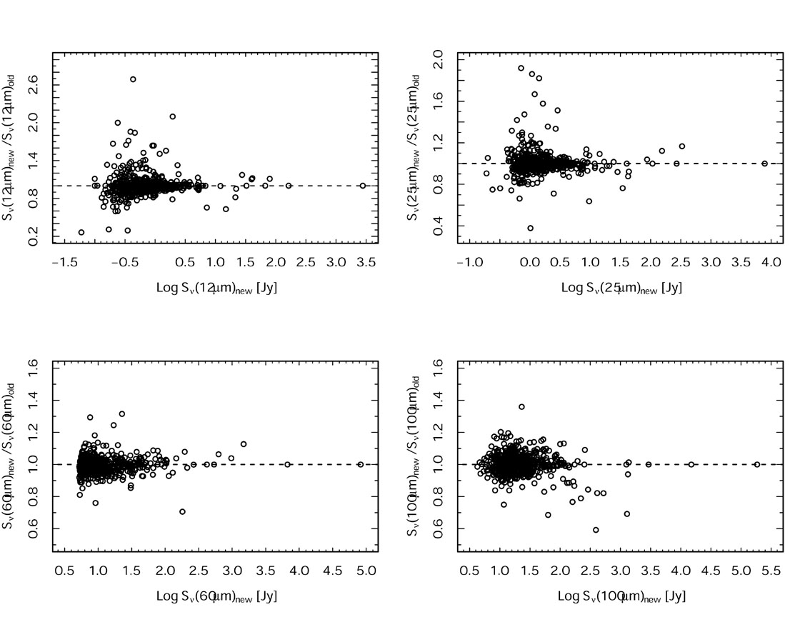 |
Figure 2. The ratio of new total flux density measurements to original estimates versus the base 10 log of the new total flux density at 12 µm, 25 µm, 60 µm and 100 µm. |
All sources with extreme
S(new)
/ S(old)
flux ratios in Figure 2 were examined in detail,
and they are explained by various improvements
in the revised processing. Some objects with
S(new)
/ S(old)
< 0.8 are cases where the RBGS flux densities have been estimated by
using
SCLEAN (see Appendix) or peak values to
minimize confusion from companion
galaxies in pairs, nearby stars, or cirrus, where in BGS1 +
BGS2 the
f(t)
method was used and therefore the flux densities quoted there were
contaminated (over estimated). Examples are NGC 5194 and NGC 5195, where SCLEAN was used
in RBGS to separate the components of this galaxy pair (M 51) at 12
µm and 25 µm. Another example is
IRAS F16516-0948 at 100 µm
(S(new)/
S(old) =
0.75), where cirrus confusion has been minimized
by using the peak flux estimate in RBGS, and
f(t)
was contaminated
(resulting in an over estimated flux density) in BGS2. Most
objects with
S(new)/
S(old) >
1.2 are cases where the RBGS flux
selection algorithm resulted in the choice of
f(t)
or f(z)
over f(template), where in BGS1 +
BGS2 a lower flux density estimate was made for
reasons explained in the previous paragraph (also see the
Appendix). Examples are NGC 3147 at 12 µm
(S(new) /
S(old) =
2.10) and MCG +07 -23 -019 at 25 µm
(S(new) /
S(old) = 1.92).
Other extreme ratios are due simply to differences between the
f(t)
results obtained using the final (PASS3) IRAS archive calibration
versus the earlier versions utilized in BGS1 +
BGS2; an example is NGC 4565 at 60 µm
(S(new) /
S(old) =
0.79). Most of the remaining outliers in
Figure 2 are explained by the use of the SCANPI
f(z)
measurement for all
objects smaller than 25 arcminutes in size, where in BGS1 +
BGS2 flux measurements from Rice et al.
(1983;
1988)
were always used when available. Examples are
NGC 134 at 60 µm
(S(new) /
S(old) =
1.32) and NGC 4631
at 100 µm
(S(new) /
S(old) =
0.77). As discussed in
Section 2, comparison of the Rice et
al. measurements with SCANPI
f(z)
measurements for galaxies with optical sizes less than 25 arcminutes
showed relatively uniform scatter in the residuals, indicating that the use
of SCANPI
f(z),
when significantly larger than
f(t),
is the
best choice for these objects to insure uniformity and consistency in the
calibration with the rest of the RBGS objects.
Figure 3 shows the ratio of total flux density
to the peak flux density in
the coadded scans at 12 µm, 25 µm, 60
µm and 100 µm. The
f(peak)
value is used here rather than
f(template) because
the latter measurement does not exist for objects in which the point source
template (PSF) fit failed, while for pure point sources
f(total)
 f(template) and thus the ratio
S(total) /
S(peak) is very
close to unity. This figure illustrates the degree to which point-source
fitted measurements in the IRAS PSC and IRAS FSC
underestimate the total
flux densities for objects in the RBGS. There are likely numerous errors in
the literature concerning the infrared flux densities and infrared colors
of galaxies, due to the fact that some users of IRAS data have
not fully appreciated the fact that most bright infrared galaxies in the
local universe, as represented here in the RBGS, are marginally extended
or resolved by IRAS.
f(template) and thus the ratio
S(total) /
S(peak) is very
close to unity. This figure illustrates the degree to which point-source
fitted measurements in the IRAS PSC and IRAS FSC
underestimate the total
flux densities for objects in the RBGS. There are likely numerous errors in
the literature concerning the infrared flux densities and infrared colors
of galaxies, due to the fact that some users of IRAS data have
not fully appreciated the fact that most bright infrared galaxies in the
local universe, as represented here in the RBGS, are marginally extended
or resolved by IRAS.
 |
Figure 3. Ratio of the best estimate of the total flux density to the peak value in the coadded scan vs the base 10 log of the new total flux density at 12 µm, 25 µm, 60 µm and 100 µm. Only a few objects with very large ratios are outside the plot region; the selected range in the ratio was chosen to show details for the largest number of points. |
A summary of the percentages of sources that were found to be extended in
each of the IRAS bands in given in
Table 5. The most notable result is that
at 60 µm and 100 µm, where S/N is highest and
distinctions can be reliably made, there are significantly more
resolved or marginally resolved objects than previously thought: 48% in
the RBGS versus 45% as previously reported in the BGS1 +
BGS2 at 60 µm, and 30% in the RBGS versus 23% as
previously reported in
the BGS1 + BGS2 at 100 µm.
This is due to a more careful definition of resolved or marginally
extended objects as those having significantly more flux between the
baseline zero-crossings,
f(z),
than within the nominal detector size,
f(t),
in combination with a comparison of W25 and W50 measurements to
point-source values. We should emphasize that the
BGS1 + BGS2 used only
W25 and W50 to determine whether sources are resolved, and always chose
f(t)
to estimate the flux for the R and M (U+) objects.
The revised processing has resulted in significantly fewer objects with
underestimated total fluxes in the RBGS compared to BGS1 +
BGS2.
| Detection Type | 12µm | 25µm | 60µm | 100µm |
| RBGS Resolveda - R | 338 (54%) | 266 (42%) | 219 (35%) | 81 (13%) |
| BGS1+BGS2 Resolved - R | 349 (56%) | 321 (52%) | 195 (32%) | 72 (12%) |
| RBGS Marginally Resolveda - M | 43 (7%) | 77 (12%) | 82 (13%) | 105 (17%) |
| BGS1+BGS2 Marginally Resolved - U+ | 84 (14%) | 112 (18%) | 80 (13%) | 71 (11%) |
| RBGS Unresolveda - U | 229 (36%) | 286 (46%) | 328 (52%) | 443 (70%) |
| BGS1+BGS2 Unresolved - U | 179 (29%) | 185 (30%) | 343 (55%) | 471 (76%) |
| RBGS Upper Limits | 19 (3%) | 0 | 0 | 0 |
| RBGS Uncertain fluxesb | 34 (5%) | 37 (6%) | 40 (6%) | 59 (9%) |
| † The number and approximate percentages of objects in each category are listed. The RBGS contains 629 objects and BGS1 + BGS2 contains 618 objects. | ||||
| a IRAS scan profile size information as identified with the size code (S) following each flux density and uncertainty listed in Table 1. See the description of columns (8) - (11) in Table 1, and Figure 14 (Appendix) for examples of coadded scan profiles that illustrate size codes "R", "M", and "U". | ||||
| b Various types of measurement uncertainties as encoded in the flag (F) following some flux density and uncertainty values listed in Table 1. See the description of columns (8) - (11) in Table 1, and Figure 16 (Appendix) for examples of scan profiles that illustrate the uncertainty flags "g", "b", "c", and "n". | ||||