APPENDIX

Data Reduction and Detailed SCANPI Measurements

Many sources in the RBGS are near enough such that they appear resolved or marginally extended in one or more of the IRAS detector bands, while others are unresolved. Therefore, an objective and consistent procedure had to be developed to select the best estimate of the total flux density for each object in each of the four IRAS bands. Table 7 lists the IRAS SCANPI measurements for all sources in the RBGS; these data were used along with the coadded scan plots to determine the "best" flux density estimates as listed in Table 1. These measurements are from the SCANPI median (1002) method of IRAS scan coaddition (Helou et al. 1988). Table 7 includes the coaddition results from all four SCANPI methods ("zc", "tot", "template", "peak") for each source in the RBGS. Our automated processing methods selected the final flux densities listed in Table 1 based on the relative values from these four coadd methods, plus the use of important additional information concerning source extent, and possible confusion due to blended sources, companions, Galactic cirrus, or excessive noise. Examples of how these choices were made are illustrated in Figures 14 - 16, and more thoroughly discussed in the captions to these figures.

The column entries in Table 7 are as follows:

(1) Name - The Common name as listed in Table 1.

(2) Redshift Reference - 19 digit reference code from NED for the redshift listed in Table 1.

(3) N/O - Ratio of the new IRAS flux density estimate to the old flux density estimate published previously in BGS₁ or BGS₂ at 12 µm; objects new to the RBGS have missing values ("--") in this and following columns.

(4) zc - flux density from SCANPI's zero-crossing measurement, f(z) (Jy) at 12 µm.

(5) tot - flux density from SCANPI's in-band total measurement, f(t) (Jy) at 12 µm.

(6) temp - flux density from SCANPI's template amplitude measurement, tmpamp (Jy) at 12 µm.

(7) peak - flux density from SCANPI's peak measurement, peak (Jy) at 12 µm.

(8) W25 - scan profile full width (arcminutes) measured at 25% of the peak signal at 12 µm.

(9) W50 - scan profile full width (arcminutes) measured at 50% of the peak signal at 12 µm.

(10-16) - Same measurements as in columns (3) - (9), but at 25µm.

(17-23) - Same measurements as in columns (3) - (9), but at 60µm.

(24-30) - Same measurements as in columns (3) - (9), but at 100µm.

Table 7 in data format.

Table 7 in postscript format.

For some objects, values of temp are 0.00 or values of W25 and W50 are negative in Table 7. These are indications that the point source template amplitude fit failed, which occurred for some very extended objects best measured using the f(z) flux estimator; see the example of NGC 1532 at 25 µmplotted in panel (a) of Figure 15.

Perhaps of most immediate interest to those familiar with the previous BGS₁ + BGS₂ datat are the N/O values given in columns (3), (10), (17) and (24) of Table 7. Part of the differences in the "new" versus "old" flux densities is simply that due to the improved "Pass 3" calibration adopted for the final release of the IRAS Level1 Archive. However, a significant effect is that due to the improved methods of estimating the total flux, in particular the use of f(z) when this flux measurement was significantly larger than the other coadd methods due to extended emission not captured by f(t). In addition, as mentioned in Section 4.1, many galaxies have profile widths which are not significantly broader than what is expected for a point source, yet there is extended emission in a faint "pedestal" can be easily seen in the profiles, and reliably measured as a statistically significant excess of the f(t) aperture value over the f(template) point source fitted value. Figure 13 shows the distribution of the ratio f(t) / f(template) at 60 µm; also plotted are Gaussian fits intended to model the distribution expected solely from noise in the relative f(t) and f(template) measurements for unresolved objects, data for a sample of comparably bright stars, and 60 µm profiles for representative RBGS objects. This information was used as follows to establish the threshold for when f(t) could be selected as a reliable, confident indicator of extended emission in excess of the value measured by the point source template fit.

A sample of candidate stars was selected from the IRAS Point Source Catalog (PSC) using the joint criteria of f(60µm) > 5.24 Jy, a high point source fit correlation coefficient (99%), and positional association with objects in one or more star catalogs. The resulting candidate list (195 objects) was further filtered by cross-identification of each IRAS source with known stars using information available in SIMBAD. Some are planetary nebulae or unknown object types and were therefore omitted for this purpose of identifying a large sample of pure 60 µm point sources. The remaining sample of confirmed stars were then processed with SCANPI using the same procedure as the RBGS objects. The distribution of the measured ratios of f(t) / f(template) for 121 confirmed bright stars with high quality 60 µm IRAS scans (e.g., not confused by cirrus, excessive noise, or companions) is plotted in the same bins as the RBGS objects in Figure 13 (asterisks). The presence of stars with ratios greater than ~ 1.05 was unexpected, and this complicated the goal of building a comparison sample of pure IRAS 60 µm point sources; close inspection of the data showed that each of these objects have 60 µm scan profiles similar to the RBGS galaxy profiles plotted in Figure 13, with faint "pedestals" faint emission under a dominating point source. Larger ratios correspond to higher or more extended pedestals well above the background noise in the scans. These are clear candidates for stars embedded in extended circumstellar dust disks, shells or nebulae; some objects have published data that support this interpretation, including spectral classifications such as carbon stars, emission-line stars, and stars with known OH/IR envelopes. These objects are not considered further in this paper, but their presence required omitting stars outside the range 0.95 - 1.05 to form a Gaussian fit representative of unresolved stars measured by SCANPI. This fitted distribution of stars (dotted line, with a mean of 1.000 ± 0.004) was then scaled to match the peak of the Gaussian fit to the RBGS objects (solid line), and plotted as a dashed line in Figure 13.

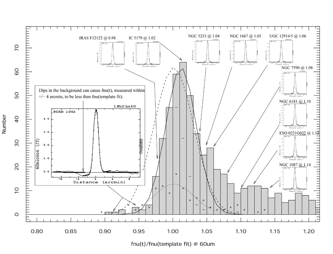Figure 13. Histogram illustrating the distribution of the ratio f(t) / f(template) at 60 µm. The entire range of this parameter is not shown in order to highlight details of the distribution for objects that have a ratio near unity. The solid line is a Gaussian fit to the upper envelop of the galaxy distribution, constructed by rejecting objects outside the range 0.95 - 1.05 from the fit. The asterisks show counts in the same bins for a sample of 121 stars selected from the IRAS Point Source Catalog (PSC) with f(60µm) > 5.24 Jy and positional associations with objects in various star catalogs; cross-identification of these IRAS sources with stars was confirmed using SIMBAD. The dotted line is a Gaussian fit to the distribution for the stars, again omitting objects outside the range 0.95 - 1.05 from the fit. The dashed line is a Gaussian distribution with the same mean and standard deviation as the fit to the star distribution (dotted line), but scaled to the peak of the galaxy distribution (solid line). Horizontal line segments have been drawn in the bins with f(t) / f(template) values between 1.0 and 1.10; these represent a "reflection" of the bins with f(t) / f(template) values between 0.90 and 1.00 for the RBGS objects, indicating the expected counts if differences between f(t) and f(template) were due only to noise and not real excess, extended emission detected in the f(t) measurement. The small plots inset around the top and right sides of the figure illustrate representative coadded 60 µm scan profiles from SCANPI; the object name and corresponding value of f(t) / f(template) at 60 µm is listed above each plot. The larger inset plot on the left illustrates how dips in the background noise cause f(t) to be less than the template fit (point spread function) value for some objects; in such cases, f(template) was chosen over f(t). This diagram was used to establish the threshold requirement of f(t) / f(template) > 1.05 for selecting f(t) as a confident measurement of at least marginally extended emission in excess of the value measured by the point source template fit.

Another approach to predicting the expected distribution for unresolved galaxies with f(t) / f(template) > 1.0 is based on the assumption that small differences between the two measurements (whether negative or positive) are due solely to noise in the coadded scans and uncertainties in the IRAS point source template fits. That is, if all galaxies with f(t) / f(template) between 1.00 and 1.10 were unresolved by IRAS at 60 µm, we would expect the observed RBGS histogram bins over this range to match a reflection of the distribution over the range 0.90 - 1.00, where differences between f(t) and f(template) are clearly not physical and therefore due solely to noise. These expected counts are shown as horizontal line segments drawn within the bins with f(t) / f(template) values between 1.0 and 1.10. Using this noise symmetry argument to predict the f(t) / f(template) ratios expected for truly unresolved objects over the range 1.0 - 1.1, there is a clear excess of galaxies with ratios as small as 1.04 - 1.05 that likely have real (but weak) extended components; roughly 50% of the RBGS objects in these bins are in this category. However, since we cannot distinguish, using visual inspection of the coadded scan profiles, between galaxies that have true extended emission and those which have f(t) > f(template) due only to noise among these objects, we cannot reliably use a threshold ratio smaller than 1.05 to classify specific objects as marginally extended. Although the bins with f(t) / f(template) in the range 1.05 - 1.10 have counts that suggest some of these objects may be explained by the Gaussian fits described above for unresolved objects, visual inspection of the SCANPI profiles shows that every object in this range (and of course larger values) have clear, obvious extended emission as shown in the example profiles inset in Figure 13. Finally, the reality of extended emission for RBGS objects with ratios f(t) / f(template) > 1.05 is visualized in Figure 13 through the progressive increase in the height or spatial extent of the pedestals corresponding to an increase in the flux ratio, all clearly defined well above the background noise in the coadded scans.

The threshold ratio of f(t) / f(template) > 1.05 (5% excess flux over the point source template fit) was therefore used for defining marginally extended objects (M). Visual examination of the coadded scan profiles widths in conjunction with the flux ratio distribution in Figure 13 lead to selection of a threshold of f(t) / f(template) > 1.20 (20% flux excess over the point source template fit) to flag a source as fully resolved (R), even if there is no additional excess flux measured by the f(z) method and therefore the f(t) value is selected. The final algorithm chosen for selecting the best SCANPI method for estimating the total flux density and for assigning IRAS source size codes in each IRAS band is as follows:

1. If the condition [f(t) > = 1.05 * f(template) AND f(t) > = f(template) + 3 * sigma] is true OR the condition [W50 > = W50_psf OR W25 > = W25_psf] is true, f(t) is selected and the source is classified as marginally extended (M). The sigma above and in other conditions that follow is the standard deviation of the coadded data measured by SCANPI in the background noise outside the signal range; these values are tabulated in columns (8) - (11) of Table 1 in units of mJy. W50_psf and W25_psf are the thresholds used to establish when a galaxy profile's width at 50% peak (FWHM) or 25% peak are significantly larger than observed among unresolved point sources. The W50_psf and W25_psf thresholds adopted, rather conservatively, are the computed mean plus 3 times the rms dispersion observed in each IRAS band for a large sample of point sources: 1.04' and 1.40' at 12 µm, 1.00' and 1.38' at 25 µm, 1.52' and 2.06' at 60 µm, and 3.22' and 4.32'at 100 µm. For reference, the nominal FWHM of the IRAS detectors is 0.77' (12 µm), 0.78' (25 µm), 1.44' (60 µm), and 2.94' (100 µm).
2. If the condition [f(t) > = 1.20 * f(template) AND f(t) > = f(template) + 3 * sigma] is true OR the condition [W50 > = W50_psf AND W25 > = W25_psf] is true, f(t) is selected and the object is classified as resolved (R).
3. If the condition [f(z) > = f(t) + 3 * sigma] is true, AND the condition [f(z) > = f(peak)] is true, AND the condition [f(z) > = 1.05 * f(t)] is true, f(z) is selected and the source is classified as resolved (R).
4. If none of the above conditions are satisfied, the f(template) method is selected and the source is classified as unresolved (U).
5. For coadded scans that display confusion from nearby sources, blends of close pairs, excessive noise, cirrus contamination, etc., based on visual inspection made for all of the data, selections resulting from the algorithm above were overridden using flags specified in the input data. For example, the peak flux value is a better estimate (flagged with method code "P" in Table 1) when the f(t) value is tainted by a bad point source template fit due to a nearby confusing source or cirrus (e.g., IRAS 02572 + 7002 at 60 µm; see Fig. 15.). Another example is when the SCLEAN algorithm was used in an attempt to de-blend components of a pair (e.g., NGC 5194 / 95 = M 51; see Fig. 15.).

Figures 14 - 16 display coadded IRAS scan profiles that illustrate the meaning of the source size codes (S), SCANPI flux density methods (M), and uncertainty flags (F) as listed for each source in Table 1.

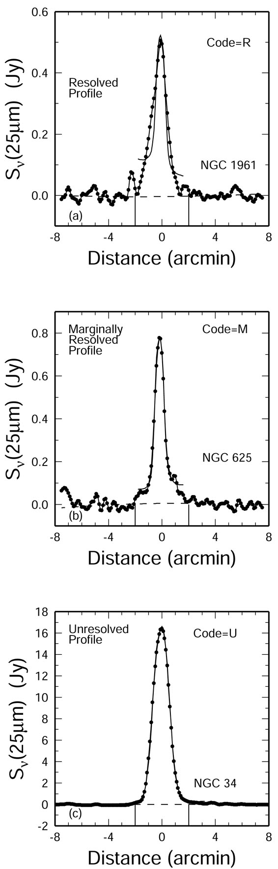Figure 14. Coadded IRAS scan profiles that illustrate source size codes listed in columns (8) - (11) of Table 1 (the "S" in "SMF"). Panel (a) R - resolved source NGC1961. Panel (b) M - marginally resolved source (called "U+" in BGS1 + BGS2) NGC625. Panel (c) U - unresolved source NGC34. In this figure, as well as in Figs. 15 and 16, the solid points are the median coadded IRAS scan data (SCANPI coadd method 1002), the dashed lines are the baseline fits to the background noise, and the solid lines are the point source template fits (point-spread function). The vertical bars below the fitted baseline show the integration range used for the total flux density estimation, f(t), which is measured within a defined region; the default SCANPI ranges for f(t) were used, which are ±2, ±2, ±2.5 and ±4 arcminutes at 12 µm, 25 µm, 60 µm and 100 µm.

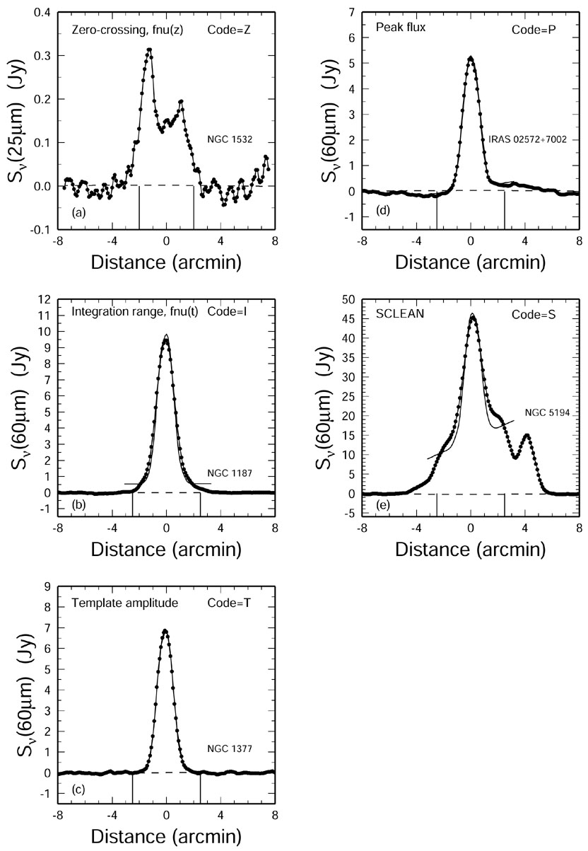Figure 15. Coadded IRAS scan profiles that illustrate flux density estimator methods listed as codes in columns (8) - (11) of Table 1 (the "M" in "SMF"). Panel (a): Z - total flux density estimated from integration of the averaged scan between the zero crossings; called "f(z)" in SCANPI output. Panel (b): I - total flux density estimated from integration of the coadded scan between fixed points defining an integration range; called "f(t)" in SCANPI output. Note the slightly raised point source template fit, which is another indicator of small, but statistically significant excess emission compared to the case of a pure point source. The default SCANPI ranges for f(t) were used, which are ±2, ±2, ±2.5 and ±4 arcminutes at 12 µm, 25 µm, 60 µm and 100 µm. Panel (c): T - flux density estimated from the best-fitting point source template; called 'template amplitude' in the SCANPI output. This is the method most often selected by the software for unresolved sources with no confusion. Note that the point source template fit is not raised with respect to the baseline fit of the background emission; this is a visual confirmation of the result found by the automated method selection - within the statistical noise, f(t) is not larger than the template fit. Panel (d): P - the maximum flux density measured within the signal range; called "peak" in SCANPI output. This method was used when emission from a nearby source or cirrus confused the template fit and contaminated the f(t) and f(z) methods. Panel (e): S - result of SCLEAN point source subtraction (see Appendix); this method was used to estimate the flux density of components of some pairs, for comparison with generally more reliable HIRES results (Surace, Sanders & Mazzarella 2003). The first four codes are referred to as "peak", "temp", "tot" and "zc", respectively, in the header of Table 7. Another value of the measurement method code listed in Table 1 is "R"; this indicates that the total flux estimate from Rice (1993) or Rice et al. (1988) was used because the SCANPI 1-D scan coaddition method does not work well for objects larger than ~ 25 arcminutes. See text for details.

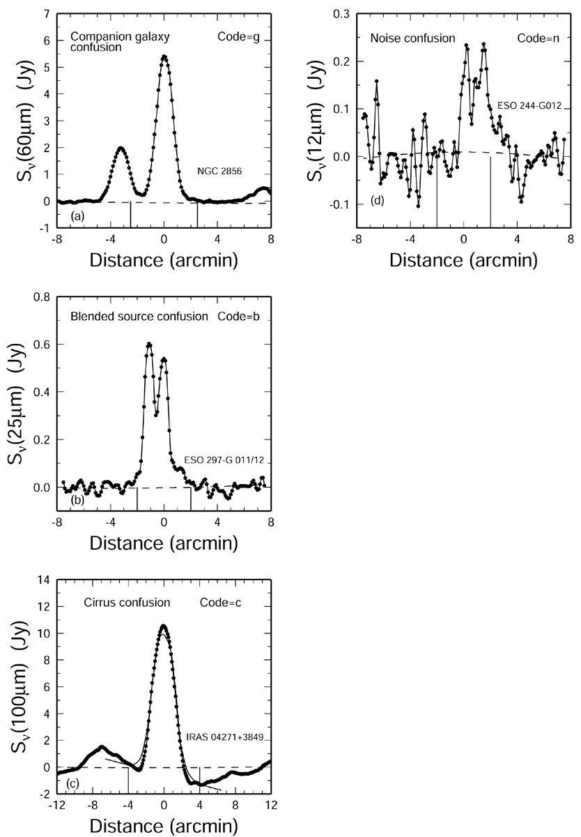Figure 16. Coadded IRAS scan profiles that illustrate uncertainty codes listed in columns (8) - (11) of Table 1 (the "F" in "SMF"). These codes identify the origin of large uncertainty flagged generally by a colon (":") following the associated flux density measurement in Table 1. Panel (a): g - a nearby companion galaxy influenced the choice of flux estimator. Panel (b): b - emission from two or more galaxies is blended; the components are unresolved by IRAS at the indicated wavelength. Panel (c): c - prominent Galactic cirrus taints the measurement. Panel (d): n - excessive noise or source confusion prevented a reliable flux density estimate.

The flux estimates chosen by the final processing are indicated by the "Method" codes following the flux densities quoted in Table 1: Z = "zero crossing" ("zc" in Table 7); I = "in-band total" ("tot" in Table 7); T = "template fit" ("temp" in Table 7); P = "peak value" ("peak" in Table 7); S = "deconvolution with SCLEAN" ¹³ ; R = from Rice et al. (1988). For objects with "R" listed as the Method code in Table 1 (objects larger than ~ 25 arcminutes) the SCANPI measurements in were not used; they are included in Table 7 just for reference.

Table 5 (Section 4.1) lists the distribution among the size codes (U,M,R) for the sources at each wavelength, and reflects primarily the changing angular resolution of the IRAS detectors as a function of wavelength, although the increased sensitivity of the IRAS detectors at 60 µm detectors compensates for the larger size of the 60 µmcompared to the smaller angular resolution of the detectors at 12 µm and 25 µm. The number of resolved or marginally resolved objects (i.e. size codes "M" or "R" respectively in Table 1) is 61% at 12 µm, 54% at 25 µm, 48% at 60 µm, and drops to 30% at 100 µm, as listed in Table 5.

¹³ SCLEAN is a simple routine that fits an IRAS point-source template at an input position and subtracts ("cleans") the fit from the 1-D coadded profile. This allows the user to estimate the flux remaining in a source which is not accounted for by point source component(s). SCLEAN was used to estimate the flux densities for components of pairs and a number of confused objects, as indicated in Table 1. Back.