Annu. Rev. Astron. Astrophys. 1996. 34: 461-510 Copyright © 1996 by Annual Reviews. All rights reserved

2.6. The First Estimates of Globular Cluster Ages

It is instructive to look back to the first papers that were written on the subject of globular cluster ages. Using hand computation, Sandage & Schwarzschild (1952) produced the first evolutionary tracks for low-mass Population II stars to somewhat beyond central hydrogen exhaustion. From these calculations they inferred an age of 3.5 × 10⁹ yr for the two globulars whose turnoffs had just been detected - M92 (Arp, Baum & Sandage 1953) and M3 (Sandage 1953). However, they had not modeled the earliest, low-luminosity phases, and when this was taken into account, the estimated age rose to 6.2 × 10⁹ yr (Hoyle & Schwarzschild 1955). Essentially the same result (6.5 Gyr) was obtained by Haselgrove & Hoyle (1956), who were the first to use a digital computer to solve the stellar structure equations.

In the 1950s, it was generally supposed that the original matter in the Galaxy was pristine (i.e. "uncooked"); consequently, the stellar models that were computed at that time assumed Y 0.0. It was not realized until somewhat later that it would be very difficult for conventional stellar nucleosynthesis to explain the increase from such low Y values to the observed high helium contents of Population I stars (see Hoyle & Tayler 1964), and it was later still that the microwave background was discovered (Penzias & Wilson 1965) and the notion that the Universe began as a singularity took hold. Big Bang nucleosynthesis calculations carried out shortly thereafter (e.g. Wagoner, Fowler & Hoyle 1967) predicted that the primordial helium abundance would be somewhere in the range 0.2 Y 0.3.

However, even before these developments, Hoyle (1959) had computed an evolutionary track for Y = 0.249 and Z = 0.001 to explore the consequences of higher Y. Because that Y, Z combination is very close to what is assumed in present-day stellar models, we thought that it would be interesting to compare the track that Hoyle computed (as tabulated in his paper) with one for the same mass (1.163 M) and chemical composition using the latest version of the University of Victoria code (see VandenBerg et al 1996). That comparison is shown in Figure 6. Considering the primitive state of our understanding of stellar physics nearly 40 years ago - even the relative importance of the pp-chain versus the CNO-cycle was largely unknown - the agreement is remarkably good. The turnoff temperatures agree to within 240 K, the turnoff luminosities to within (log L / L) = 0.05, and the turnoff ages to within 40% (4.3 Gyr for Hoyle's model versus 2.7 Gyr for ours).

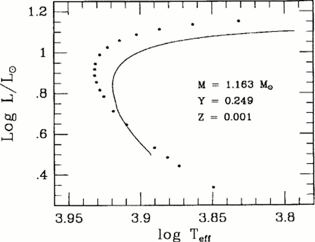Figure 6. Comparison of an evolutionary track computed by Hoyle (1959) (dotted curve) with one for the same mass and chemical composition, as specified, but using the latest version of the University of Victoria code (solid curve).

The point of this exercise is to show that the first stellar models computed for GC stars predicted a higher, not a lower, age at a fixed turnoff luminosity than do modern calculations. (The adoption of Y 0.0 would tend to further increase that age.) Therefore, the low ages reported in those initial investigations must be attributed to something other than the evolutionary models that were used. In fact, they resulted from the then conventional assumption that the RR Lyrae variables, which were used to set the GC distance scale, had M_V = 0.0. Only after such studies as that by Eggen & Sandage (1959), who used trigonometric parallax stars encompassing a range in [Fe/H] and the nearby Groombridge 1830 group of low-metallicity subdwarfs to do main-sequence fits, did it become accepted that the actual luminosities of the RR Lyraes must be near M_V = 0.5 [although there were earlier indications that this might be the case (e.g. Pavlovskaia 1953)]. Hoyle (1959) noted that this revision would imply an age for the Galaxy of greater than 10¹⁰ years. Thus, ages much more similar to current estimates would have resulted had the cluster distances been known more accurately. Even today, as we show in the next section, distance uncertainties continue to dominate over all other sources of error.