


C. Galaxy-galaxy and cluster-cluster correlations
Having re-discovered the power of the two-point correlation function as a tool for measuring clustering, it was evident that the Princeton group would go on to analyze every available catalog of extragalactic objects they could lay their hands on. One of these catalogs was the Abell catalog of rich galaxy clusters identified on the Palomar Sky Survey (Hauser and Peebles, 1973). The technique used was power spectrum analysis since it was felt this would give a better method of dealing with the incomplete sky coverage.
It came as somewhat of a surprise to discover (a) that these Abell clusters were themselves clustered and (b) that, on a given scale, they were more clustered than the galaxies. The former was a surprise because serious doubts had previously been expressed about the reality of superclustering. Here was direct evidence that clusters were likely to be found in pairs and even in groups. The latter was a surprise because it had been (naively) expected that clusters identified from a set of points would necessarily have the same correlation function as the set itself. The galaxy clusters were themselves clustered on scales where the galaxy-galaxy correlation was so small as to be immeasurable.
Both the galaxy and cluster correlation functions are
approximately power laws
 (r) =
(r / r0)-
(r) =
(r / r0)- with the
same exponent
with the
same exponent
 1.8, but the
correlation amplitudes for
clusters are much larger than those for galaxies.
1.8, but the
correlation amplitudes for
clusters are much larger than those for galaxies.
There is a simple reason why the cluster-cluster correlation function might have an amplitude exceeding the galaxy-galaxy correlation function amplitude: it arises because of the way clusters are identified as regions where groups of points have a substantially higher than average density. Such regions contain most of the close pairs that go into defining the value of the galaxy-galaxy correlation function. Moreover, eliminating the points which are not in such clusters biases the expected number of pairs that would have been found had this been a Poisson distribution containing the same number of points. The boost in the value of the correlation function achieved from such censorship depends directly on the volume of space occupied by these clusters.
This entirely obvious point was made in a preprint by Jones and Jones (1985): the paper was never published. As with many useful ideas, it became common knowledge and moved into the realm of folklore.
There remained some important questions:
It was well known that there were systematic biases in the Abell Catalog. The subsample of low richness clusters was incomplete, and the more distant clusters were systematically richer than than nearby counterparts. This was not in itself enough to remove the "discrepancy" between the galaxy-galaxy correlation function and the cluster-cluster correlation function, but it might prejudice conclusion about richness dependence of the discrepancy.
It was not until 1992 that a sufficiently good alternative to the Abell Catalog became available: this was the APM cluster catalog (Dalton et al., 1992; Dalton et al., 1997) derived from the Cambridge APM Galaxy Survey (Automatic Plate Measuring Machine) of UK Schmidt Telescope plates. Now we await results from the large 2dF and SDSS redshift catalogs which have already provided detailed information about the galaxy-galaxy correlation function.
1. Analysis of recent catalogs
Currently the best data on galaxy cluster clustering comes from redshift surveys of clusters identified in machine generated galaxy catalogs and of clusters observed in X-Ray surveys. The 2dF and SDSS surveys will undoubtedly settle this matter once and for all since they contain a large number of clusters that can be selected on the basis of redshift. However, it is already apparent (as in the Shepherd et al. (2001) study of the CNOC2 sample, for Zehavi et al. (2002) study of the Early SDSS Data, and for Madgwick et al. (2003); Norberg et al. (2001) correlation analysis of the 2dFGRS) that talking about the galaxy-galaxy correlation function is somewhat of an over-simplification in the first place: the galaxy-galaxy correlation depends strongly on the absolute magnitude, galaxy colour and galaxy spectral type. Galaxies are clearly not unbiased tracers of the underlying mass distribution.
In automated cluster searching, clusters are generally discovered via a nearest-neighbour, friends-of-friends, type of analysis. They are discovered by virtue of their central concentration and so catalogs contain clusters that are defined in terms of a "distance to your nearest neighbour" threshold length. If the threshold length is increased the catalog contains more clusters: the number of poorer, less centrally dense, clusters increases. It is not a priori obvious how the mean density of galaxies within a cluster so found relates to its central density: there will clearly be a correlation. It might well be that selecting clusters by virtue of their mean galaxy density rather than their peak density would yield different catalogs and lead to different conclusions about the systematics of cluster-cluster clustering.
It is easier to build theoretical (analytic) models based on selection by mean cluster density, ie: clusters selected via a density threshold, than it is to build models based on clusters selected by peak density. The latter requires an understanding of how the cluster dynamics works to produce the density profile of the galaxy distribution. This may contribute to some of the confusion that exists when looking for trends in the clustering of clusters.
The earlier theoretical models (Jones and Jones, 1985; Kaiser, 1984; Bahcall and West, 1992) for the clustering of clusters were based on threshold selection. The same is true of more recent hierarchical models based on multi-fractal models for the distribution of galaxies (Martínez et al., 1990; Paredes et al., 1995). Most of the conclusions about superclustering in which the clusters are defined via the peak density excursion comes from N-body simulations of various sizes and sophistication (Bahcall and Cen, 1992; Croft and Efstathiou, 1994; Colberg et al., 1998).
Since clusters found in X-ray surveys are found by virtue of their gas temperature, that is total potential, these surveys should agree rather well with the conclusions based on N-body experiments.
3. Richness dependence of the correlation length
The seminal paper on the effect of cluster richness on the cluster-cluster correlation function was that of Szalay and Schramm (1985). They suggested that the scaling length for clustering should itself depend on the cluster density. Which cluster density, peak or mean, was never stated.
The formula for the cluster two-point correlation function
(r;
 ) is usually written as
(Kaiser, 1984):
) is usually written as
(Kaiser, 1984):
 |
(26) |
where is the height of the
peaks in units of the rms error
 of the galaxy density
field, and
(r) is the
correlation function of the galaxy field
7.
of the galaxy density
field, and
(r) is the
correlation function of the galaxy field
7.
The empirical determination of the the cluster-cluster
correlation function, cc(r), is much more uncertain than
the galaxy-galaxy correlation function,
gg(r). The
selection effects associated with the cluster identification method
(Eke et al., 1996)
are the major source for this uncertainty.
The possible dependence of clustering properties on cluster
richness makes the issue still more difficult. Nevertheless
cc(r) is usually fitted to a power law
 |
(27) |
Eq. 26 holds if
c =
, where
is the
exponent of the power-law galaxy-galaxy correlation function. As
already mentioned, this seems to be the case, see for example in
Fig. 13,
the remarkable agreement between the slopes of the correlation
function of the REFLEX cluster catalog and the Las Campanas
galaxy redshift survey
(Borgani and Guzzo,
2001;
Guzzo, 2002).
Nevertheless, depending on the analyzed cluster sample and cluster
identification procedure, the scatter of the reported values for
the slope of the correlation function is very high with
c
= 1.6 to 2.5. For the correlation length the values go from
13h-1 Mpc to 40 h-1 Mpc
(Bahcall and West,
1992;
Dalton et al., 1994;
Nichol et al., 1992;
Postman et
al., 1992;
Borgani and Guzzo,
2001).
Fig. 14 illustrates this
variability displaying the differences between the correlation
function of the Abell and APM cluster samples.
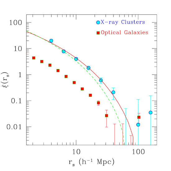 |
Figure 13. The two-point correlation function for the X-ray selected clusters from the REFLEX survey (circles) and for the Las Campanas galaxy redshift survey (squares). The solid and dashed lines are the expected results for an X-ray similar survey in a LCDM model with different values for the cosmological parameters, from Borgani and Guzzo (2001). |
Rich clusters have many members and are rare, therefore the
distance between then
dc = nc-1/3 is larger.
Bahcall and
West (1992) derived a linear relation between the
cluster correlation length rc and the mean intercluster
separation dc,
rc = 0.4dc from power-law fits
(constrained to have a fixed value of
c
= 1.8) to correlation functions
calculated on cluster samples with different richness.
Fig. 15 shows that this relation is not
confirmed by the new data. In fact, at large values of
dc the relation must
level off, and a weaker dependence of rc versus
dc agrees better with the observations, for example
rc = 2.6(dc)1/2
as shown in the figure
(Bahcall et
al., 2003).
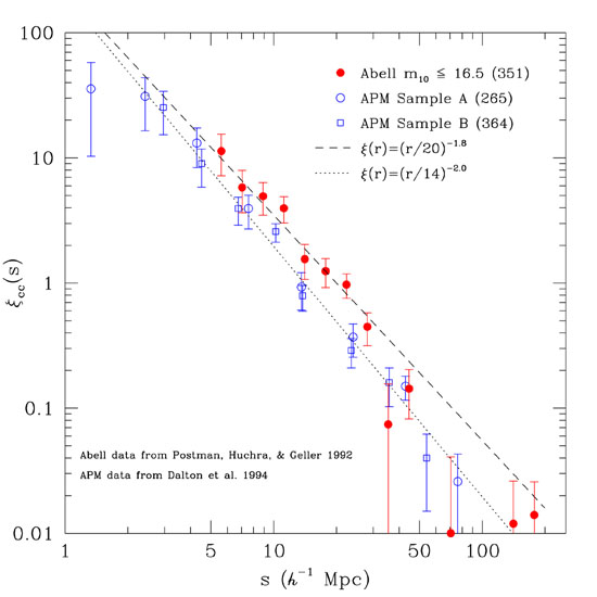 |
Figure 14. The two-point correlation functions for the Abell clusters and two subsamples of the APM survey. The best power-law fits are shown in the plot, from Postman (1999). |
Since rc and
c are not independent, the slope is
usually constrained to a fixed value
c
= 1.8. Dependence of
c
on cluster richness has been proposed
(Martínez et al.,
1995),
although this dependence is better parametrized by
the correlation dimension - the exponent of the power law
fitting the correlation integral
N(r) = A rD2 (see Eq. 16).
Multiscaling is the term used for scaling laws in which D2
displays a slowly varying behavior with the density threshold that
characterizes the richness of clusters. The higher the threshold,
the richer the clusters, and the smaller the value of D2.
Within the multiscaling framework, the relation r0
versus dc
gets a more complicated form flattening for large values of
dc as the observations confirm
Martínez et
al., 1995).
 |
Figure 15. The correlation length of different cluster samples as a function of the intercluster distance. The solid line shows the relation rc = 2.6(dc)1/2 that fits well the observations and the LCDM model, from Bahcall et al. (2003). |
7 As the correlation functions and
are defined for the density
contrast  =
(
=
( -
-
 / , all
quantities in (26) are dimensionless; there is no dimensionality conflict.
Back.
/ , all
quantities in (26) are dimensionless; there is no dimensionality conflict.
Back.