B. The correlation function: galaxies

1. Definitions and scaling

The definition of the correlation function used in cosmology differs slightly from the definition used in other fields. In cosmology we have a nonzero mean field (the mean density of the Universe) superposed on which are the fluctuations that correspond to the galaxies and galaxy clusters. Since the Universe is homogeneous on the largest scales, the correlations tend to zero on these scales.

On occasion, people have tried to use the standard definition and in doing so have come up with anomalous conclusions.

The right definition is: In cosmology, the 2-point galaxy correlation function is defined as a measure of the excess probability, relative to a Poisson distribution, of finding two galaxies at the volume elements dV₁ and dV₂ separated by a vector distance r:

(11)

where n is the mean number density over the whole sample volume. When homogeneity ⁵ and isotropy are assumed (r) depends only on the distance r = |r|. From Eq. (11), it is straightforward to derive the expression for the conditional probability that a galaxy lies at dV at distance r given that there is a galaxy at the origin of r.

(12)

Therefore, (r) measures the clustering in excess ((r) > 0) or in defect ((r) < 0) compared with a random Poisson point distribution, for which (r) = 0. It is worth to mention that in statistical mechanics the correlation function normally used is g(r) = 1 + (r) which is called the radial distribution function (McQuarrie, 1999). Statisticians call this quantity the pair correlation function (Stoyan and Stoyan, 1994). The number of galaxies, on average, lying at a distance between r and r + dr from a given one is ng(r)4 r².

A similar quantity can be defined for projected catalogs: surveys compiling the angular positions of the galaxies on the celestial sphere. The angular two-point correlation function, w(), can be defined by means of the conditional probability of finding a galaxy within the solid angle d lying at an angular distance from a given galaxy (arbitrarily chosen):

(13)

Now, is the mean number density of galaxies per unit area in the projected catalog. Since the first available catalogs were two-dimensional, with no redshift information, w() was measured before any direct measurement of (r) was possible. Nevertheless, (r) can be inferred from its angular counterpart w() by means of the Limber equation (Rubin, 1954; Limber. 1954) which provides an integral relation between the angular and the spatial correlation function for small angles,

(14)

Here y is the comoving distance and (y) is the radial selection function normalized such that (y) y² dy = 1. If (r) follows a power law (r) = (r / r₀)^-, it is straightforward to see that the angular correlation function is also a power law, w() = A ^1- (Peebles, 1980). Totsuji and Kihara (1969) were the first to derive a power-law model for (r) on the basis of the angular data. Their canonical value for the scaling exponent = 1.8 has remained unaltered for more than 30 years. Eq. 14 provides the basis for an important scaling relation. Peebles (1980) has shown that, in a homogeneous universe, w() must scale with the sample depth D_* as

(15)

where the function W is an intrinsic angular correlation function which does not depend on the apparent limmiting magnitude of the sample. The characteristic depth D_* is the distance at which a galaxy with intrinsic luminosity L_* is seen at the limiting flux density f, which is in the Euclidean geometry (neglecting expansion and curvature),

(16)

or, in terms of magnitudes,

(17)

where m₀ is the apparent limiting magnitude of the sample. The scaling relation in Eq. (15) can be deduced from the Limber equation (14) assuming that distribution of galaxies is homogeneous on average and therefore D_*³. Peebles (1993) has shown that the analysis of the deep catalogs of galaxies on the basis of the scaling law (Eq. 15) argues strongly against an unbounded self-similar fractal distribution of galaxies. In the 1970's and early 1980's a number of catalogs going to a variety of magnitude limits were available and analysed by Peebles and his collaborators. Because of the way the galaxy luminosity function works, most of the galaxies in a catalog fall within a relatively narrow range of distance that depends on the limiting magnitude of the catalog: catalogs reaching to fainter magnitudes are probing the Universe at greater distances.

As the distance increases, the angular scale subtended by a given physical distance decreases. Hence, if the Universe is homogeneous, the two-point angular correlation function of one catalog should look like a rescaled version of the two point angular correlation function of a deeper catalog (see Eq. 15), i.e., for catalogs with varying characteristic distance w D_*^-1 at a given angular separation D_*; or, in other words, if we calculate the angular correlation function on two samples, with characteristic depths D_* and D_*', Eq. 15 implies that w'((D_* / D_*') ) = (D_* / D_*') w(). The scaling relationship can be predicted precisely, though for catalogs that probe to very great depths it is necessary to be careful of K-corrections and geometric effects due to the cosmological model (Colombo and Bonometto, 2001).

The earliest catalogs available were the de Vaucouleurs catalog of Bright Galaxies, the Zwicky catalog, the Shane-Wirtanen catalog and the Jagellonian Field. Matching their correlation functions provided the first direct evidence for large scale cosmic homogeneity (Groth and Peebles, 1977; Groth and Peebles, 1986). The scaling relation has been confirmed with more recent catalogs, in particular, the APM galaxy survey has povided one of the strongest observational evidences supporting this law (Maddox et al., 1990b; Baugh, 1996; Maddox et al., 1996).

Now we can do much better since we have bigger and better catalogs with partial or complete redshift information. Such catalogs can be divided into magnitude slices and the same test performed on the two point angular correlation function of the slices. The result (Connolly et al., 2002) reproduced in Fig. 9 is as good a vindication of the homogeneity of the Universe as one could wish for. More data will be forthcoming from the 2dF and SDSS surveys.

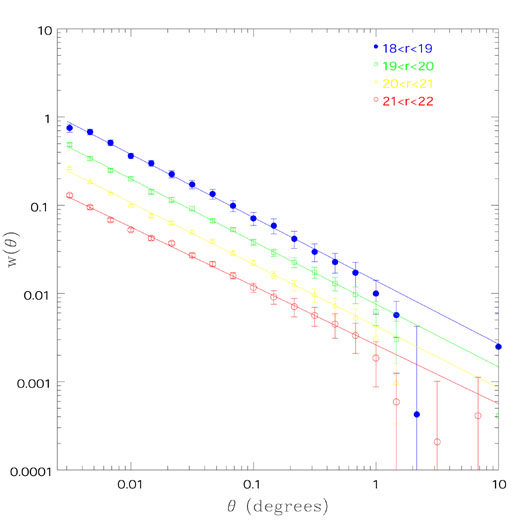Figure 9. The angular correlation function from the SDSS as a function of magnitude from Connolly et al. (2002). The correlation function is determined for the magnitude intervals 18 < r* < 19, 19 < r* < 20, 20 < r* < 21 and 21 < r* < 22. The fits to these data, over angular scales of 1' to 30', are shown by the solid lines.

The scaling properties of the correlation function are usually shown in the form of the correlation integral. For a point distribution the integral expresses the number of neighbors, on average, that an object has within a sphere of radius r. It is given by

(18)

The distribution is said to follow fractal scaling if within a large range of scales the behavior of N( < r) can be well fitted to a power law

(19)

or, alternatively

(20)

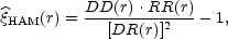
where D₂ is the so-called correlation dimension. The scaling range has to be long enough to talk about fractal behavior. However, the term has been used very often for describing scaling behaviors within rather limited scale ranges (Avnir et al., 1998). In Sect. V.B.4 we show recent determinations of D₂ for several galaxy samples at different scale ranges.

2. Estimators

The two-point correlation function (r) can be estimated in several ways from a given galaxy sample. For a discussion of them see, for example, Kerscher et al. (2000); Martinez and Saar (2002); Pons-Borderia et al. (1999). At small distances, nearly all the estimators provide very similar performance, however at large distances, their performance is not equivalent any more and some of them could be biased. Considering the galaxy distribution as a point process, the two-point correlation function at a given distance r is estimated by counting and averaging the number of neighbors each galaxy has at a given scale. It is clear that the boundaries of the sample have to be considered, because as no galaxies are observed beyond the boundaries, the number of neighbors is systematically underestimated at larger distances. If we do not make any assumption regarding the kind of point process that we are dealing with, the only solution is to use the so-called minus-estimators, the kind of estimators favored by Piertonero and co-workers (Sylos Labini et al., 1998): The averages of the number of neighbors at a given distance are taken omitting those galaxies lying closer to the border than r. At large scales only a small fraction of the galaxies in the sample enters in the estimation, increasing the variance. To make full use of the surveyed galaxies, the estimator has to incorporate an edge-correction. 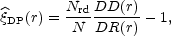The most widely used estimators in cosmology are the Davis and Peebles estimator (Davis and Peebles, 1983), the Hamilton estimator (Hamilton, 1993b), and the Landy and Szalay estimator (Landy and Szalay, 1993). Here we provide their formulae when applied to a complete galaxy sample in a given volume with N objects. A Poisson catalog, a binomial process with N_rd points, has to be generated within the same boundaries.

(21)

(22)

(23)

where DD(r) is the number of pairs of galaxies with separation within the interval [r - dr / 2, r + dr / 2, DR(r) is the number of pairs between a galaxy and a point of the Poisson catalog, and RR(r) is the number of pairs with separation in the same interval in the Poisson catalog. At large scales the performance of the Hamilton and Landy and Szalay estimators has been proved to be better (Pons-Bordería et al., 1999; Kerscher et al., 2000).

3. Recent determinations of the correlation function

Earlier estimates of the pairwise galaxy correlation function were obtained from shallow samples, and one could suspect that they were not finding the true correlation function. The first sample deep enough to get close to solving that problem was the Las Campanas Redshift Survey (LCRS). The two-point correlation function for LCRS was determined by Tucker et al. (1997) and by Jing et al. (1998) (see Fig. 10). Jing el al. get slightly smaller values for the correlation length (r₀ = 5.1 h^-1 Mpc) than Tucker et al. (r₀ = 6.3 h^-1 Mpc). When making comparisons, it is necessary to take care that the length scales have been interpreted in the same underlying cosmological model. Older papers tend to set = 0 whereas more recent papers are often phrased in terms of a flat- plus cold dark matter cosmology.

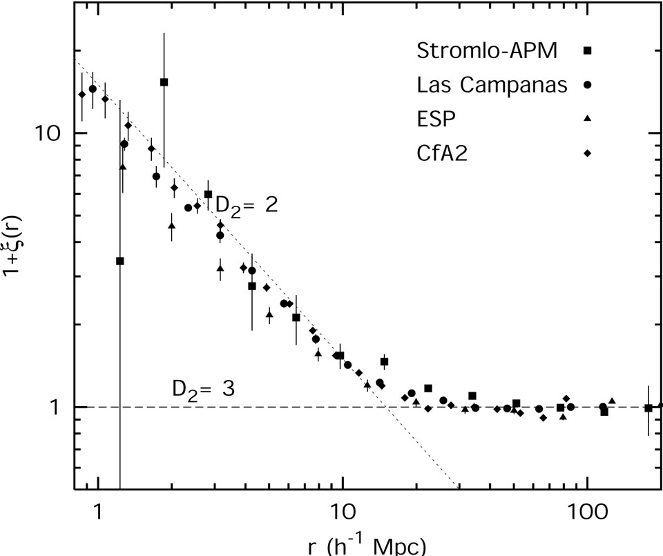Figure 10. The correlation function 1 + (r) for different samples calculated with different estimators. We can see that the small scale fractal regime is followed by a gradual transition to homogeneity.

Analyzing data from the first batch of the SSDS, Zehavi et al. (2002) analyse 29300 galaxies covering a 690 square degree region of sky, made up of a number of long narrow segments (2.5 - 5 degrees). They arrive at an average real-space correlation function of

(24)

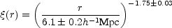
for 0.1 h^-1 Mpc < r < 16 h^-1 Mpc. This comes close to the LCRS result of Tucker et al. (1997). More recently, the same group (Zehavi et al., 2003) has updated the result, using a more complete sample with 118,149 galaxies (see Fig. 11), and the best power-law fit is

(25)

This is a remarkable scaling law covering some 3 orders of magnitude in distance. The smallest scale measured (100 h^-1 kpc) is barely larger than a typical galaxy. Interestingly, this lower scale is set, in the Zehavi et al. (2002) analysis, by the requirement that, at the outer limit of the survey (corresponding to a radial velocity of 39,000 km s^-1), pairs of galaxies should be no closer than can be reached by two neighboring fibers on the multifiber system. There would be some interest in looking at nearer galaxies and tracing the correlation function to even smaller scales to see whether the old and remarkable extrapolation of Gott and Turner (1979) ⁶ is valid in this newer data set (see also Infante et al. (2002)). The largest distance (16 h^-1 Mpc) is larger than the size of a great cluster. It should be emphasized that this is a real space correlation function: the finger-of-god effects have been filtered.

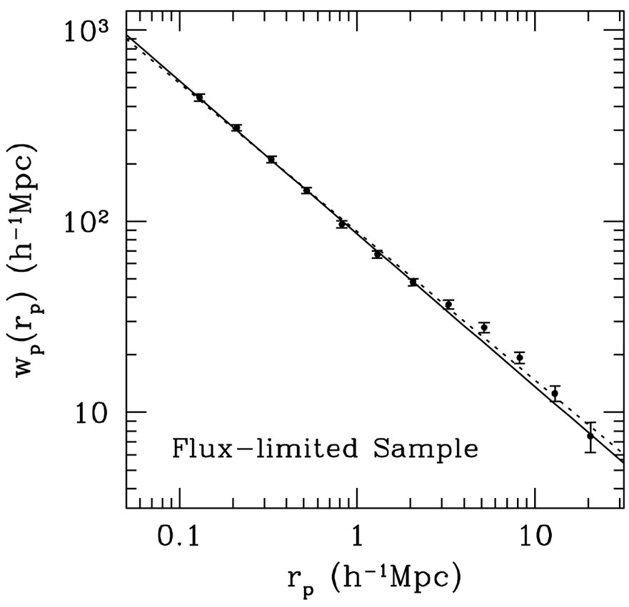Figure 11. The (projected) real space two point-correlation function of the SSDS data from Zehavi et al. (2003). The two straight lines show different fits corresponding to different weighting schemes

There is a substantial luminosity effect seen in the scale length. The absolute magnitude M_* of the "knee" of the Schechter galaxy luminosity function (Schechter, 1976) is taken as a reference point (being a "typical" galaxy luminosity, whatever that means). For galaxies with absolute magnitudes centered on M_* - 1.5 the scale length is r₀ 7.4 h^-1 Mpc. For samples centered on M_* the scale length is r₀ 6.3 h^-1 Mpc. And for samples centered on M_* + 1.5 the scale length is r₀ 4.7 h^-1 Mpc. The slope for these samples is essentially the same. A similar strong dependence of the correlation function on the color, morphology, and redshift of galaxies was found before, in the Canadian Network for Observational Cosmology Field Galaxy Redshift Survey (CNOC2) by Shepherd et al. (2001).

The angular correlation function for the SDSS (Connolly et al., 2002) is independent of redshift distortions and agrees well with the value inferred from the redshift survey. This encourages one to believe that the redshift corrections are being handled effectively.

However, the latest careful analysis of the (almost) full 2dF survey (Hawkins et al., 2003) gives the correlation length r₀ = 5.05 h^-1 Mpc, substantially smaller than the SDSS result. Hawkins et al. (2003) ascribe this to the different galaxy content of the two surveys: the SDSS is a red-magnitude selected survey and the 2dFGRS is a blue magnitude selected survey.

4. Correlation dimension

Recently, many authors have measured the correlation dimension of the galaxy distribution at different scales using all available redshift catalogs. Wu et al. (1999) and Kurokawa et al. (2001) summarized these results in a table. A more completed and updated version of a similar table, including more references and new catalogs is presented here (see Table I). The estimates of the correlation dimension have been performed using different methods depending on the authors' preferences. It is worthwhile to mention the elegant technique introduced by Amendola and Palladino (1999) based on radial cells that maximizes the scale at which the minus-estimator can be applied. The table shows unambiguously that the correlation dimension is a scale dependent quantity, increasing gradually from values D₂ 2 for scales less than 20 - 30 h^-1 Mpc (and even larger values of D₂ in IRAS based redshift surveys) to values approaching D₂ 3 for larger scales.

Table I. The correlation dimension estimated on different redshift surveys at different scale ranges.

Reference	Sample	Range of scales (h-1 Mpc)	D2
Martínez and Jones, 1990	CfA-I	3-10	1.15 - 1.40
Lemson and Sanders, 1991	CfA-I	1 - 30	2
Domínguez-Tenreiro et al., 1994	CfA-I	1.5 - 25	2
Kurokawa et al., 1999	CfA-II	7 - 27	1.89 ± 0.06
Guzzo et al., 1991	Perseus-Pisces	1 - 3.5	1.25 ± 0.10
	Perseus-Pisces	3.5 - 27	2.21 ± 0.06
	Perseus-Pisces	27 - 70	3
Martínez et al., 1998	Perseus-Pisces	1 - 20	1.8 - 2.3
Martínez and Coles, 1994	QDOT	1 - 10	2.25
	QDOT	10 - 50	2.77
Martínez et al., 1998	Stromlo-APM	30 - 60	2.7 - 2.9
Hatton, 1999	Stromlo-APM	12 - 55	2.76
Amendola and Palladino, 1999	Las Campanas	20 - 30	2
	Las Campanas	> 30	3
Kurokawa et al., 2001	Las Campanas	5 - 32	1.96 ± 0.05
	Las Campanas	32 - 63	3
Pan and Coles, 2000	PSCz	< 10	2.16
	PSCz	10 - 30	2.71
	PSCz	30 - 400	2.99

5. Correlation length as a function of sample depth

The first indication that correlation length might depend on the sample depth was found in the CfA-I data (Einasto et al., 1986). The correlation length increased, when deeper samples were chosen. Although the authors explained the effect by the specific geometry of the mass distribution in shallow samples, this paper motivated the early campaign to explain the galaxy distribution as fractals (Calzetti et al., 1988; Pietronero, 1987), because for a fractal r₀ increases proportionally with the sample depth (Coleman and Pietronero, 1992; Guzzo, 1997). The Ruffini group realized from the beginning that fractal scaling cannot extend to large scales and started to look for crossover to homogeneity (Calzetti et al., 1991), but the Pietronero group has continued the fractal war until now, fighting for an all-fractal universe. Their stand is summarized in Sylos and Labini et al. (1998).

The deep samples now at our disposal have solved this problem once and for all - the galaxy correlation functions may depend on their intrinsic properties (luminosity, morphology, etc.), but not on the sample size (Martínez et al., 2001; Kerscher, 2003). As an example, Fig. 12 shows the results of a recent study.

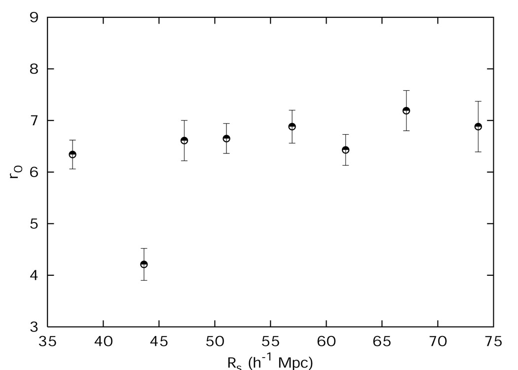Figure 12. The correlation length as a function of the sample depth for the CfA-II catalog, from Martinez et al. (2001). The observed plateau argues against the fractal interpretation of the galaxy distribution.

⁵ This property is called stationarity in point field statistics. Back.

⁶ Gott and Turner estimated the small-scale end of the correlation function down to a scale of 30 h^-1 kpc from the distribution of projected distances between isolated galaxy pairs (double galaxies). As strange as it may seem, this correlation function fitted neatly the general galaxy correlation function. Back.