H. Generalizations: IV. Jets

The afterglow theory becomes much more complicated if the relativistic ejecta is not spherical. The commonly called "jets" corresponds to relativistic matter ejected into a cone of opening angle . I stress that unlike other astrophysical jets this ejecta is non steady state and generally its width (in the direction parallel to the motion) is orders of magnitude smaller than the radius where the jet is. A "flying pancake" is a better description for these jets.

The simplest implication of a jet geometry, that exists regardless of the hydrodynamic evolution, is that once ~ ^-1 relativistic beaming of light will become less effective. The radiation was initially beamed locally into a cone with an opening angle ^-1 remained inside the cone of the original jet. Now with ^-1 > the emission is radiated outside of the initial jet. This has two effects: (i) An "on axis" observer, one that sees the original jet, will detect a jet break due to the faster spreading of the emitted radiation. (ii) An "off axis" observer, that could not detect the original emission will be able to see now an "orphan afterglow", an afterglow without a preceding GRB (see Section VIIK). The time of this transition is always give by Eq. 104 below with C₂ = 1.

Additionally the hydrodynamic evolution of the source changes when ~ ^-1. Initially, as long as >> ^-1 [305] the motion would be almost conical. There isn't enough time, in the blast wave's rest frame, for the matter to be affected by the non spherical geometry, and the blast wave will behave as if it was a part of a sphere. When = C₂ ^-1, namely at ⁸:

(103)

sideways propagation begins. The constant C₁ expresses the uncertainty at relation between the Lorentz factor and the observing time and it depends on the history of the evolution of the fireball. The constant C₂ reflects the uncertainty in the value of , when the jet break begins vs. the value of opening angle of the jet . For the important case of constant external density k = 0 this transition takes place at:

(104)

The sideways expansion continues with ~ ^-1. Plugging this relations in Eq. 78 and letting vary like ^-2 one finds that:

(105)

A more detailed analysis [204, 309, 343, 344] reveals that according to the simple one dimensional analytic models decreases exponentially with R on a very short length scale. ⁹

Table VI describes the parameters and for a post jet break evolution [374]. The jet break usually takes place rather late, after the radiative transition. Therefore, I include in this table only the slow cooling parameters.

Table VI. and for slow cooling (_a < _m < _c) after a jet break.

< a	0	2
a < < m	-1/3	1/3
m < < c	-p	- (p - 1) / 2 = ( + 1) / 2
c <	-p	- p / 2 = /2

An important feature of the post jet-break evolution is that _c, the cooling frequency becomes constant in time. This means that the high frequency (optical and X-ray) optical spectrum does not vary after the jet-break took place. On the other hand the radio spectrum varies (see Fig. 25), giving an additional structure that confirms the interpretation of break as arising due to a sideways expansion of a jet (see e.g. [159]).

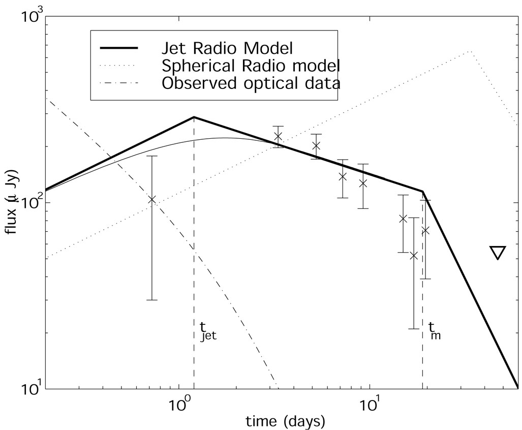Figure 25. Observed and predicted light curve at 8.6 Ghz light curves of GRB 990510 (from Harrison et al. [159]). The different behavior of the optical and radio light curves after the jet break is clearly seen.

Panaitescu and Kumar [290] find that the jet break transition in a wind profile will be very long (up to four decades in time) and thus it will be hard to observe a jet break in such a case. On the other hand it is interesting to note that for typical values of seen after a jet break ( - 2) the high frequency spectral index, = / 2 - 1, is similar to the one inferred from a spherically symmetric wind = (2 + 1) / 3 - 1 [157]. Note however, that the wind interpretation requires a high ( 3) p value (which may or may not be reasonable). Still from the optical observations alone it is difficult to distinguish between these two interpretations. Here the radio observations play a crucial role as the radio behavior is very different [106].

The sideways expansion causes a change in the hydrodynamic behavior and hence a break in the light curve. The beaming outside of the original jet opening angle also causes a break. If the sideways expansion is at the speed of light than both transitions would take place at the same time [374]. If the sideways expansion is at the sound speed then the beaming transition would take place first and only later the hydrodynamic transition would occur [292]. This would cause a slower and wider transition with two distinct breaks, first a steep break when the edge of the jet becomes visible and later a shallower break when sideways expansion becomes important.

The analytic or semi-analytic calculations of synchrotron radiation from jetted afterglows [204, 264, 292, 344, 374] have led to different estimates of the jet break time t_jet and of the duration of the transition. Rhoads [344] calculated the light curves assuming emission from one representative point, and obtained a smooth `jet break', extending ~ 3 - 4 decades in time, after which F _{> m} t^-p. Sari et al. [374] assume that the sideways expansion is at the speed of light, and not at the speed of sound (c / 3^1/2) as others assume, and find a smaller value for t_jet. Panaitescu and Mészáros [292] included the effects of geometrical curvature and finite width of the emitting shell, along with electron cooling, and obtained a relatively sharp break, extending ~ 1 - 2 decades in time, in the optical light curve. Moderski et al. [264] used a slightly different dynamical model, and a different formalism for the evolution of the electron distribution, and obtained that the change in the temporal index (F t^-) across the break is smaller than in analytic estimates ( = 2 after the break for > _m, p = 2.4), while the break extends over two decades in time.

The different analytic or semi-analytic models have different predictions for the sharpness of the `jet break', the change in the temporal decay index across the break and its asymptotic value after the break, or even the very existence a `jet break' [171]. All these models rely on some common basic assumptions, which have a significant effect on the dynamics of the jet: (i) the shocked matter is homogeneous (ii) the shock front is spherical (within a finite opening angle) even at t > t_jet (iii) the velocity vector is almost radial even after the jet break.

However, recent 2D hydrodynamic simulations [137] show that these assumptions are not a good approximation of a realistic jet. Using a very different approach Cannizzo et al. [48] find in another set of numerical simulations a similar result - the jet does not spread sideways as much. Figure 26 shows the jet at the last time step of the simulation of Granot et al. [137]. The matter at the sides of the jet is propagating sideways (rather than in the radial direction) and is slower and much less luminous compared to the front of the jet. The shock front is egg-shaped, and quite far from being spherical. Figure 27 shows the radius R, Lorentz factor , and opening angle of the jet, as a function of the lab frame time. The rate of increase of with R ct_lab, is much lower than the exponential behavior predicted by simple models [204, 309, 343, 344]. The value of averaged over the emissivity is practically constant, and most of the radiation is emitted within the initial opening angle of the jet. The radius R weighed over the emissivity is very close to the maximal value of R within the jet, indicating that most of the emission originates at the front of the jet ¹⁰, where the radius is largest, while R averaged over the density is significantly lower, indicating that a large fraction of the shocked matter resides at the sides of the jet, where the radius is smaller. The Lorentz factor averaged over the emissivity is close to its maximal value, (again since most of the emission occurs near the jet axis where is the largest) while averaged over the density is significantly lower, since the matter at the sides of the jet has a much lower than at the front of the jet. The large differences between the assumptions of simple dynamical models of a jet and the results of 2D simulations, suggest that great care should be taken when using these models for predicting the light curves of jetted afterglows. Since the light curves depend strongly on the hydrodynamics of the jet, it is very important to use a realistic hydrodynamic model when calculating the light curves.

Figure 26. A relativistic jet at the last time step of the simulation [137]. (left) A 3D view of the jet. The outer surface represents the shock front while the two inner faces show the proper number density (lower face) and proper emissivity (upper face) in a logarithmic color scale. (right) A 2D 'slice' along the jet axis, showing the velocity field on top of a linear color-map of the lab frame density.

Figure 27. The radius R (left frame), Lorentz factor - 1 (middle frame) and opening angle of the jet (right frame), as a function of the lab frame time in days [137].

Granot et al. [137] used 2D numerical simulations of a jet running into a constant density medium to calculate the resulting light curves, taking into account the emission from the volume of the shocked fluid with the appropriate time delay in the arrival of photons to different observers. They obtained an achromatic jet break for > _m(t_jet) (which typically includes the optical and near IR), while at lower frequencies (which typically include the radio) there is a more moderate and gradual increase in the temporal index at t_jet, and a much more prominent steepening in the light curve at a latter time when _m sweeps past the observed frequency. The jet break appears sharper and occurs at a slightly earlier time for an observer along the jet axis, compared to an observer off the jet axis (but within the initial opening angle of the jet). The value of after the jet break, for > _m, is found to be slightly larger than p ( = 2.85 for p = 2.5). Due to the fact that a significant fraction of the jet break occurs due to the relativistic beaming effect (that do not depend on the hydrodynamics) in spite of the different hydrodynamic behavior the numerical simulations show a jet break at roughly the same time as the analytic estimates.

⁸ The exact values of the uncertain constants C₂ and C₁ are extremely important as they determine the jet opening angle (and hence the total energy of the GRB) from the observed breaks, interpreted as t_jet, in the afterglow light curves. Back.

⁹ Note that the exponential behavior is obtained after converting Eq. 74 to a differential equation and integrating over it. Different approximations used in deriving the differential equation lead to slightly different exponential behavior, see [309]. Back.

¹⁰ This may imply that the expected rate of orphan afterglows should be smaller than estimated assuming significant sideways expansion! Back