


2.6. Kron magnitudes
Kron (1980) presented the following luminosity-weighted radius, R1, which defines the `first moment' of an image
| (31) |
He argued that an aperture of radius twice R1, when R1 is obtained by integrating to a radius R that is 1% of the sky flux, contains more than ~ 90% of an object's total light, making it a useful tool for estimating an object's flux.
It is worth noting that considerable confusion exists in the
literature in regard to the definition of R1. To help
avoid ambiguity, we point out that g(x) in
Kron's (1980)
original equation refers to xI(x), where x is the
radius and I(x) the intensity profile.
Infante (1987)
followed this notation, but confusingly a
typo appears immediately after his Equation 3 where he has written
g(x) ~ I(x) instead of
g(x) ~ xI(x). Furthermore, Equation 3
of Bertin & Arnouts
(1996)
is given as R1 =
 RI(R) /
I(R) where the
summation is over a two-dimensional aperture
rather than a one-dimensional light-profile. In the latter case,
one would have
R1 =
R2 I(R) /
RI(R).
RI(R) /
I(R) where the
summation is over a two-dimensional aperture
rather than a one-dimensional light-profile. In the latter case,
one would have
R1 =
R2 I(R) /
RI(R).
Using a Sérsic intensity profile, and substituting in x = b(R / Re)1/n, the numerator can be written as
|
Using Equation (2) for the denominator, which is simply the enclosed luminosity, Equation (31) simplifies to
| (32) |
The use of `Kron radii' to determine `Kron magnitudes' has proved very popular, and SExtractor (Bertin & Arnouts 1996) obtains its magnitudes using apertures that are 2.5 times R1. Recently, however, it has been reported that such an approach may, in some instances, be missing up to half of a galaxy's light (Bernstein, Freedman, & Madore 2002; Benitez et al. 2004). If the total light is understood to be that coming from the integration to infinity of a light-profile, then what is important is not the sky-level or isophotal-level one reaches, but the number of effective radii that have been sampled.
For a range of light-profiles shapes n, Figure (8) shows the value of R1 (in units of Re) as a function of the number of effective radii to which Equation (31) has been integrated. Given that one usually only measures a light-profile out to 3-4 Re at best, one can see that only for light-profiles with n less than about 1 will one come close to the asymptotic value of R1 (i.e, the value obtained if the profile was integrated to infinity). Table (1) shows these asymptotic values of R1 as a function of n, and the magnitude enclosed within 2R1 and 2.5R1. This is, however, largely academic because observationally derived values of R1 will be smaller than those given in Table (1), at least for light-profiles with values of n greater than about 1.
 |
Figure 8. Kron radii R1, as obtained from Equation (32), are shown as a function of the radius R to which the integration was performed. Values of n range from 0.5, 1, 2, 3,... 10. |
| Sérsic n | R1 | L( < 2R1) | L( < 2.5R1) |
| [Re] | % | % | |
| 0.5 | 1.06 | 95.7 | 99.3 |
| 1.0 | 1.19 | 90.8 | 96.0 |
| 2.0 | 1.48 | 87.5 | 92.2 |
| 3.0 | 1.84 | 86.9 | 90.8 |
| 4.0 | 2.29 | 87.0 | 90.4 |
| 5.0 | 2.84 | 87.5 | 90.5 |
| 6.0 | 3.53 | 88.1 | 90.7 |
| 7.0 | 4.38 | 88.7 | 91.0 |
| 8.0 | 5.44 | 89.3 | 91.4 |
| 9.0 | 6.76 | 90.0 | 91.9 |
| 10.0 | 8.39 | 90.6 | 92.3 |
From Figure (8) one can see, for example, that an R1/4 profile integrated to 4Re will have R1 = 1.09Re rather than the asymptotic value of 2.29Re. Now 2.5 × 1.09Re encloses 76.6% of the object's light rather than 90.4% (see Table 1). This is illustrated in Figure (9) where one can see when and how Kron magnitudes fail to represent the total light of an object. This short-coming is worse when dealing with shallow images and with highly concentrated systems having large values of n (brightest cluster galaxies are known to have Sérsic indices around 10 or greater, Graham et al. 1996).
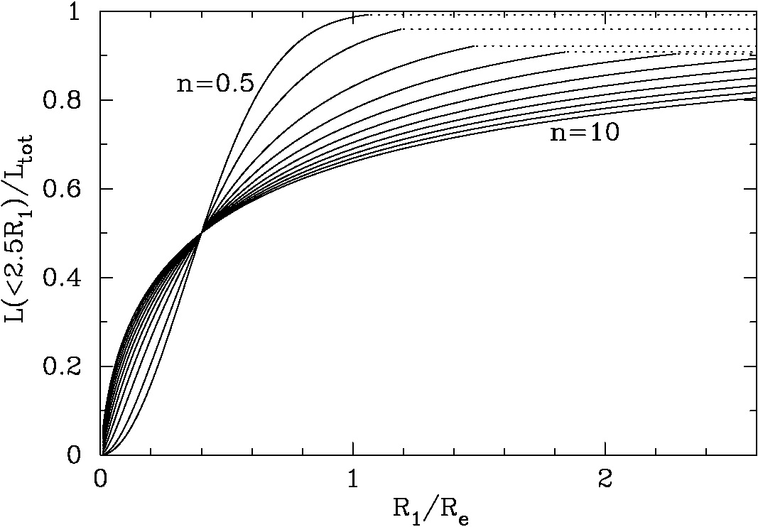 |
Figure 9. Kron luminosity within 2.5R1, normalised against the total luminosity, as a function of how many effective radii R1 corresponds to. Values of n range from 0.5, 1, 2, 3,... 10. |
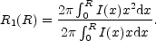
To provide a better idea of the flux fraction represented by Kron magnitudes, and one which is more comparable with Figure (7), Figure (10) shows this fraction as a function of light-profile shape n. The different curves result from integrating Equation (31) to different numbers of effective radii in order to obtain R1. If n=4, for example, but one only integrates out to 1Re (where Re is again understood to be the true, intrinsic value rather than the observed value), then the value of R1 is 0.41Re and the enclosed flux within 2.5R1 is only 50.7%. If an n = 10 profile is integrated to only 1Re, then R1 = 0.30Re and the enclosed flux is only 45.0% within 2.5R1. It is therefore easy to understand why people have reported Kron magnitudes as having missed half of an object's light.
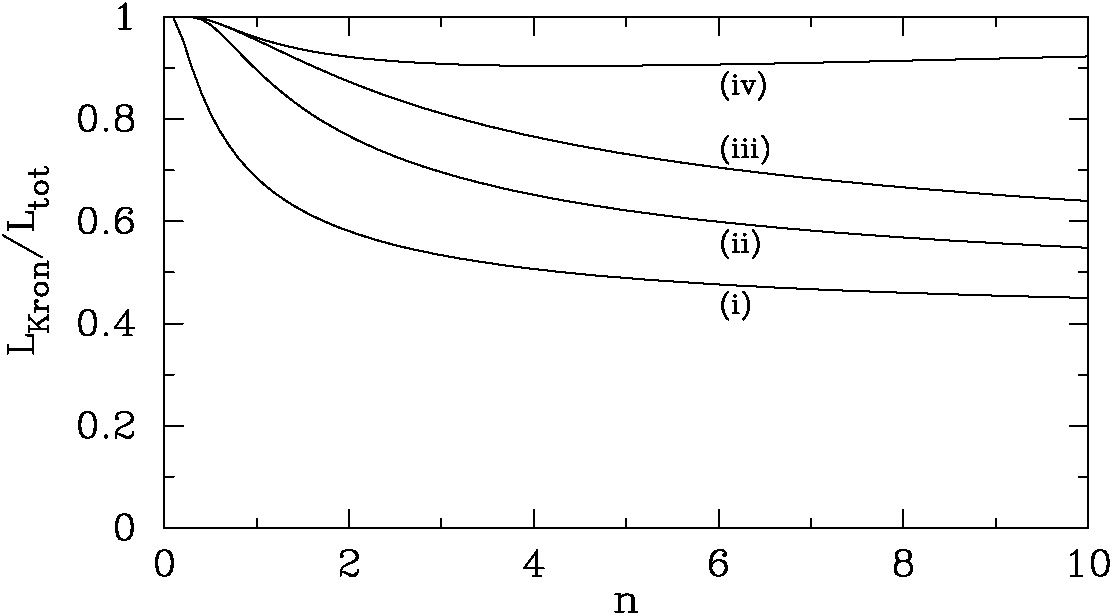 |
Figure 10. Kron luminosity within 2.5R1, normalised against the total luminosity, as a function of the underlying light-profile shape n. The different curves arise from the different values of R1 obtained by integrating Equation (31) to (i) 1Re, (ii) 2Re, (iii) 4Re, and (iv) infinity. |