1. ROLE OF OBSERVATIONS IN COSMOLOGY & GALAXY FORMATION

1.1. The Observational Renaissance

These are exciting times in the field of cosmology and galaxy formation! To justify this claim it is useful to review the dramatic progress made in the subject over the past 25 years. I remember vividly the first distant galaxy conference I attended: the IAU Symposium 92 Objects of High Redshift, held in Los Angeles in 1979. Although the motivation was strong and many observers were pushing their 4 meter telescopes to new limits, most imaging detectors were still photographic plates with efficiencies of a few percent and there was no significant population of sources beyond a redshift of z = 0.5, other than some radio galaxies to z 1 and more distant quasars.

In fact, the present landscape in the subject would have been barely recognizable even in 1990. In the cosmological arena, convincing angular fluctuations had not yet been detected in the cosmic microwave background nor was there any consensus on the total energy density _TOT. Although the role of dark matter in galaxy formation was fairly well appreciated, neither its amount nor its power spectrum were particularly well-constrained. The presence of dark energy had not been uncovered and controversy still reigned over one of the most basic parameters of the Universe: the current expansion rate as measured by Hubble's constant. In galaxy formation, although evolution was frequently claimed in the counts and colors of galaxies, the physical interpretation was confused. In particular, there was little synergy between observations of faint galaxies and models of structure formation.

In the present series of lectures, aimed for non-specialists, I hope to show that we stand at a truly remarkable time in the history of our subject, largely (but clearly not exclusively) by virtue of a growth in observational capabilities. By the standards of all but the most accurate laboratory physicist, we have `precise' measures of the form and energy content of our Universe and a detailed physical understanding of how structures grow and evolve. We have successfully charted and studied the distribution and properties of hundreds of thousands of nearby galaxies in controlled surveys and probed their luminous precursors out to redshift z 6 - corresponding to a period only 1 Gyr after the Big Bang. Most importantly, a standard model has emerged which, through detailed numerical simulations, is capable of detailed predictions and interpretation of observables. Many puzzles remain, as we will see, but the progress is truly impressive.

This gives us confidence to begin addressing the final frontier in galaxy evolution: the earliest stellar systems and their influence on the intergalactic medium. When did the first substantial stellar systems begin to shine? Were they responsible for reionizing hydrogen in intergalactic space and what physical processes occurring during these early times influenced the subsequent evolution of normal galaxies?

Let's begin by considering a crude measure of our recent progress. Figure 1 shows the rapid pace of discovery in terms of the relative fraction of the refereed astronomical literature in two North American journals pertaining to studies of galaxy evolution and cosmology. These are cast alongside some milestones in the history of optical facilities and the provision of widely-used datasets. The figure raises the interesting question of whether more publications in a given field means most of the key questions are being answered. Certainly, we can conclude that more researchers are being drawn to work in the area. But some might argue that new students should move into other, less well-developed, fields. Indeed, the progress in cosmology, in particular, is so rapid that some have raised the specter that the subject may soon reaching some form of natural conclusion (c.f. Horgan 1998).

Figure 1. Fraction of the refereed astronomical literature in two North American journals related to galaxy evolution and the cosmological parameters. The survey implies more than a doubling in fractional share over the past 15 years. Some possibly-associated milestones in the provision of unique facilities and datasets are marked (courtesy: J. Brinchmann).

1.2. Observations Lead to Surprises

It's worth emphasizing that many of the key features which define our current view of the Universe were either not anticipated by theory or initially rejected as unreasonable. Here is my personal short list of surprising observations which have shaped our view of the cosmos:

1. The cosmic expansion discovered by Slipher and Hubble during the period 1917-1925 was not anticipated and took many years to be accepted. Despite the observational evidence and the prediction from General Relativity for evolution in world models with gravity, Einstein maintained his preference for a static Universe until the early 1930's.

2. The hot Big Bang picture received widespread support only in 1965 upon the discovery of the cosmic microwave background (Penzias & Wilson 1965). Although many supported the hypothesis of a primeval atom, Hoyle and others considered an unchanging `Steady State' universe to be a more natural solutuion.

3. Dark matter was inferred from the motions of galaxies in clusters over seventy years ago (Zwicky 1933) but no satisfactory explanation of this puzzling problem was ever presented. The ubiquity of dark matter on galactic scales was realized much later (Rubin et al 1976). The dominant role that dark matter plays in structure formation only followed the recent observational evidence (Blumenthal et al 1984). ¹

4. The cosmic acceleration discovered independently by two distant supernovae teams (Riess et al 1998, Perlmutter et al 1999) was a complete surprise (including to the observers, who set out to measure the deceleration). Although the cosmological constant, , had been invoked many times in the past, the presence of dark energy was completely unforeseen.

Given the observational opportunities continue to advance. it seems reasonable to suppose further surprises may follow!

1.3. Recent Observational Milestones

Next, it's helpful to examine a few of the most significant observational achievements in cosmology and structure formation over the past 15 years. Each provides the basis of knowledge from which we can move forward, eliminating a range of uncertainty across a wide field of research.

The Rate of Local Expansion: Hubble's Constant

The Hubble Space Telescope (HST) was partly launched to resolve the puzzling dispute between various observers as regards to the value of Hubble's constant H₀, normally quoted in kms sec^-1 Mpc^-1, or as h, the value in units of 100 kms sec^-1 Mpc^-1. During the planning phases, a number of scientific key projects were defined and proposals invited for their execution.

A very thorough account of the impasse reached by earlier ground-based observers in the 1970's and early 1980's can be found in Rowan-Robinson (1985) who reviewed the field and concluded a compromise of 67 ± 15 kms sec^-1 Mpc^-1, surprisingly close to the presently-accepted value. Figure 2 nicely illustrates the confused situation.

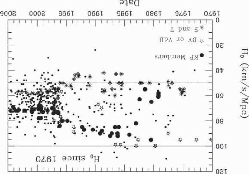Figure 2. Various values of Hubble's constant in units of kms sec-1 Mpc-1 plotted as a function of the date of publication. Labels refer to estimates by Sandage & Tammann, de Vaucouleurs, van den Bergh and their respective collaborators. Estimates from the HST Key Project group (Freedman et al 2001) are labeled KP. From an initial range spanning 50 < H0 < 100, a gradual convergence to the presently-accepted value is apparent. (Plot compiled and kindly made available by J. Huchra)

Figure 3 shows the two stage `step-ladder' technique used by Freedman et al (2001) who claim a final value of 67 ± 15 kms sec<sup>-1</sup> Mpc<sup>-1</sup>. `Primary' distances were estimated to a set of nearby galaxies via the measured brightness and periods of luminous Cepheid variable stars located using HST's WFPC-2 imager. Over the distance range across which such individual stars can be seen (<25 Mpc), the leverage on H₀ is limited and seriously affected by the peculiar motions of the individual galaxies. At 20 Mpc, the smooth cosmic expansion would give V_exp 1400 kms sec^-1 and a 10% error in H₀ would provide a comparable contribution, at this distance, to the typical peculiar motions of galaxies of V_pec 50-100 kms sec^-1. Accordingly, a secondary distance scale was established for spirals to 400 Mpc distance using the empirical relationship first demonstrated by Tully & Fisher (1977) between the I-band luminosity and rotational velocity. At 400 Mpc, the effect of V_pec is negligible and the leverage on H₀ is excellent. Independent distance estimators utilizing supernovae and elliptical galaxies were used to verify possible systematic errors.

Figure 3. Two step approach to measuring Hubble's constant H0 - the local expansion rate (Freedman et al 2001). (Left) Distances to nearby galaxies within 25 Mpc were obtained by locating and monitoring Cepheid variables using HST's WFPC-2 camera; the leverage on H0 is modest over such small distances and affected seriously by peculiar motions. (Right) Extension of the distance-velocity relation to 400 Mpc using the I-band Tully-Fisher relation and other techniques. The absolute scale has been calibrated using the local Cepheid scale.

The second significant milestone of the last 15 years is the improved understanding of the cosmic microwave background (CMB) radiation, commencing with the precise black body nature of its spectrum (Mather et al 1990) indicative of its thermal origin as a remnant of the cosmic fireball, and the subsequent detection of fluctuations (Smoot et al 1992), both realized with the COBE satellite data. The improved angular resolution of later ground-based and balloon-borne experiments led to the isolation of the acoustic horizon scale at the epoch of recombination (de Bernadis et al 2000, Hanany et al 2000). Subsequent improved measures of the angular power spectrum by the Wilkinson Microwave Anisotropy Probe (WMAP, Spergel et al 2003, 2006) have refined these early observations. The location of the primary peak in the angular power spectrum at a multiple moment l 200 (corresponding to a physical angular scale of 1 degree) provides an important constraint on the total energy density _TOT and hence spatial curvature.

The derivation of spatial curvature from the angular location of the first acoustic (or `Doppler') peak, _H, is not completely independent of other cosmological parameters. There are dependences on the scale factor via H₀ and the contribution of gravitating matter _M, viz:

where h is H₀ in units of 100 kms sec^-1 Mpc^-1.

However, in the latest WMAP analysis, combining with distant supernovae data, space is flat to within 1%.

Clustering of Galaxies: Gravitational Instability

Galaxies represent the most direct tracer of the rich tapestry of structure in the local Universe. The 1970's saw a concerted effort to introduce a formalism for describing and interpreting their statistical distribution through angular and spatial two point correlation functions (Peebles 1980). This, in turn, led to an observational revolution in cataloging their distribution, first in 2-D from panoramic photographic surveys aided by precise measuring machines, and later in 3-D from multi-object spectroscopic redshift surveys.

The angular correlation function w() represents the excess probability P of finding a pair of galaxies separated by an angular separation (degrees).

In a catalog averaging N galaxies per square degree, the probability of finding a pair separated by can be written:

where is the solid angle of the counting bin, (i.e. to + ).

The corresponding spatial equivalent, (r) in a catalog of mean density per Mpc³ is thus:

One can be statistically linked to the other if the overall redshift distribution of the sources is available.

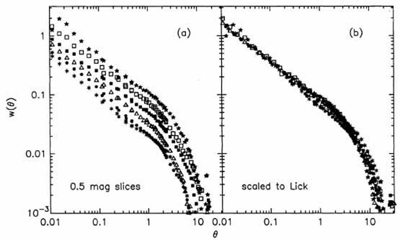Figure 4. Angular correlation function for the APM galaxy catalog - a photographic survey of the southern sky (Maddox et al 1990) - partitioned according to limiting magnitude (left). The amplitude of the clustering decreases with increasing depth due to an increase in the number of uncorrelated pairs and a smaller projected physical scale for a given angle. These effects can be corrected in order to produce a high signal/noise function scaled to a fixed depth clearly illustrating a universal power law form over nearly 3 dex (right).

Figure 4 shows a pioneering detection of the angular correlation function w() for the Cambridge APM Galaxy Catalog (Maddox et al 1990). This was one of the first well-constructed panoramic 2-D catalogs from which the large scale nature of the galaxy distribution could be discerned. A power law form is evident:

where, for example, is measured in degrees. The amplitude A decreases with increasing depth due to both increased projection from physically-uncorrelated pairs and the smaller projected physical scale for a given angle.

Figure 5. Galaxy distribution from the completed 2dF redshift survey (Colless et al 2001).

Highly-multiplexed spectrographs such as the 2 degree field instrument on the Anglo-Australian Telescope (Colless et al 2001) and the Sloan Digital Sky Survey (York et al 2001) have led to the equivalent progress in 3-D surveys (Figure 5). In the early precursors to these grand surveys, the 3-D equivalent of the angular correlation function, was also found to be a power law:

where r_o (Mpc) is a valuable clustering scale length for the population.

As the surveys became more substantial, the power spectrum P(k) has become the preferred analysis tool because its form can be readily predicted for various dark matter models. For a given density field (x), the fluctuation over the mean is = / and for a given wavenumber k, the power spectrum becomes:

The final power spectrum for the completed 2dF survey is shown in Figure 6 (Cole et al 2005) and is in remarkably good agreement with that predicted for a cold dark matter spectrum consistent with that which reproduces the CMB angular fluctuations.

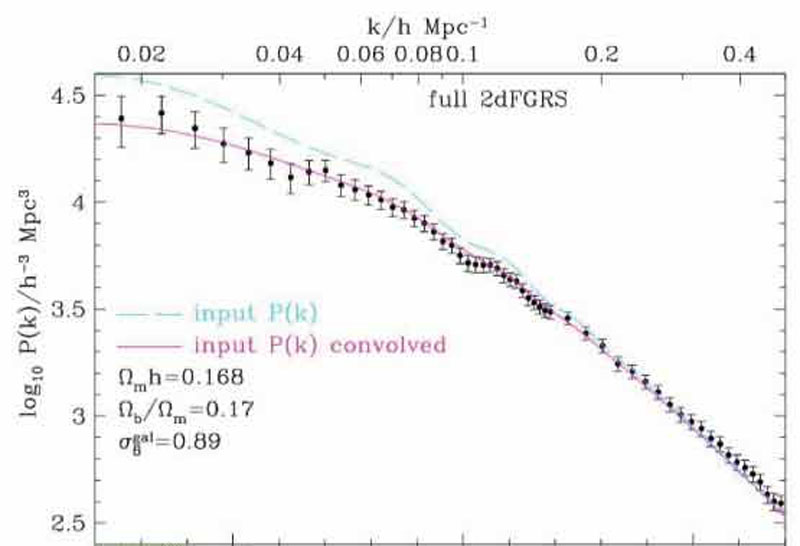Figure 6. Power spectrum from the completed 2dF redshift survey (Cole et al 2005). Solid lines refer to the input power spectrum for a dark matter model with the tabulated parameters and that convolved with the geometric `window function' which affects the observed shape on large scales.

We have already mentioned the ubiquity of dark matter on both cluster and galactic scales. The former was recognized as early as the 1930's from the high line of sight velocity dispersion _los of galaxies in the Coma cluster (Zwicky 1933). Assuming simple virial equilibrium and isotropically-arranged galaxy orbits, the cluster mass contained with some physical scale R_cl is:

which far exceeds that estimated from the stellar populations in the cluster galaxies. High cluster masses can also be confirmed completely independently from gravitational lensing where a background source is distorted to produce a `giant arc' - in effect a partial or incomplete `Einstein ring' whose diameter _E for a concentrated mass M approximates:

and D = D_sD_l, / D_ds where the subscripts s and l refer to angular diameters distances of the background source and lens respectively.

On galactic scales, extended rotation curves of gaseous emission lines in spirals (see review by Rubin 2000) can trace the mass distribution on the assumption of circular orbits, viz:

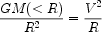Flat rotation curves (V ~ constant) thus imply M(< R) R. Together with arguments based on the question on the stability of flattened disks (Ostriker & Peebles 1973), such observations were critical to the notion that all spiral galaxies are embedded in dark extensive `halos'.

The evidence for halos around local elliptical galaxies is less convincing largely because there are no suitable tracers of the gravitational potential on the necessary scales (see Gerhard et al 2001). However, by combining gravitational lensing with stellar dynamics for intermediate redshift ellipticals, Koopmans & Treu (2003) and Treu et al (2006) have mapped the projected dark matter distribution and show it to be closely fit by an isothermal profile (r) r^-2.

The presence of dark matter can also be deduced statistically from the distortion of the galaxy distribution viewed in redshift space, for example in the 2dF survey (Peacock et al 2001). The original idea was discussed by Kaiser et al (1987). The spatial correlation function (r) is split into its two orthogonal components, (, ) where represents the projected separation perpendicular to the line of sight (unaffected by peculiar motions) and is the separation along the line of sight (inferred from the velocities and hence used to measure the effect). The distortion of (, ) in the direction can be measured on various scales and used to estimate the line of sight velocity dispersion of pairs of galaxies and hence their mutual gravitational field. Depending on the extent to which galaxies are biased tracers of the density field, such tests indicate _M = 0.25.

On the largest scales, weak gravitational lensing can trace the overall distribution and dark matter content of the Universe (Blandford & Narayan 1992, Refregier 2003). Recent surveys are consistent with these estimates (Hoekstra et al 2005).

Dark Energy and Cosmic Acceleration

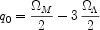
Prior to the 1980's observational cosmologists were obsessed with two empirical quantities though to govern the cosmic expansion history - R(t): Hubble's constant H₀ = dR / dt and a second derivative, the deceleration parameter q₀, which would indicate the fate of the expansion:

In the presence only of gravitating matter, Friedmann cosmologies indicate _M = 2 q₀. The distant supernovae searches were begun in the expectation of measuring q₀ independently of _M and verifying a low density Universe.

As we have discussed, Type Ia supernovae (SNe) were found to be fainter at a given recessional velocity than expected in a Universe with a low mass density; Figure 7 illustrates the effect for the latest results from the Canada-France SN Legacy Survey (Astier et al 2006). In fact the results cannot be explained even in a Universe with no gravitating matter! A formal fit for q₀ indicates a negative value corresponding to a cosmic acceleration.

Acceleration is permitted in Friedmann models with a non-zero cosmological constant . In general (Caroll et al 1992):

where = / 8 G is the energy density associated with the cosmological constant.

Figure 7. Hubble diagram (distance-redshift relation) for calibrated Type Ia supernovae from the first year data taken by the Canada France Supernova Legacy Survey (Astier et al 2006). Curves indicate the relation expected for a high density Universe without a cosmological constant and that for the concordance cosmology (see text)

The appeal of resurrecting the cosmological constant is not only its ability to explain the supernova data but also the spatial flatness in the acoustic peak in the CMB through the combined energy densities _M + - the so-called Concordance Model (Ostriker & Steinhardt 1996, Bahcall et al 1999).

However, the observed acceleration raises many puzzles. The absolute value of the cosmological constant cannot be understood in terms of physical descriptions of the vacuum energy density, and the fact that _M implies the accelerating phase began relatively recently (at a redshift of z 0.7). Alternative physical descriptions of the phenomenon (termed `dark energy') are thus being sought which can be generalized by imagining the vacuum obeys an equation of state where the negative pressure p relates to the energy density via an index w,

in which case the dependence on the scale factor R goes as

The case w = -1 would thus correspond to a constant term equivalent to the cosmological constant, but in principle any w < -1/3 would produce an acceleration and conceivably w is itself a function of time. The current SNLS data indicate w = -1.023 ± 0.09 and combining with the WMAP data does not significantly improve this constraint.

1.4. Concordance Cosmology: Why is such a curious model acceptable?

According to the latest WMAP results (Spergel et al 2006) and the analysis which draws upon the progress reviewed above (the HST Hubble constant Key Project, the large 2dF and SDSS redshift surveys, the CFHT supernova survey and the first weak gravitational lensing constraints), we live in a universe with the constituents listed in Table 1.

Table 1: Cosmic Constituents

Total Matter	M	0.24 ± 0.03
Baryonic Matter	B	0.042 ± 0.004
Dark Energy		0.73 ± 0.04

Secondly, the above parameters reconcile the growth of structure from the CMB to the local redshift surveys in exquisite detail. Numerical simulations based on 10¹⁰ particles (e.g. Springel et al 2005) have reached the stage where they can predict the non-linear growth of the dark matter distribution at various epochs over a dynamic range of 3-4 dex in physical scales. Although some input physics is needed to predict the local galaxy distribution, the agreement for the concordance model (often termed CDM) is impressive. In short, a low mass density and non-zero both seem necessary to explain the present abundance and mass distribution of galaxies. Any deviation would either lead to too much or too little structure.

This does not mean that the scorecard for CDM should be considered perfect at this stage. As discussed, we have little idea what the dark matter or dark energy might be. Moreover, there are numerous difficulties in reconciling the distribution of dark matter with observations on galactic and cluster scales and frequent challenges that the mass assembly history of galaxies is inconsistent with the slow hierarchical growth expected in a -dominated Universe. However, as we will see in later lectures, most of these problems relate to applications in environments where dark matter co-exists with baryons. Understanding how to incorporate baryons into the very detailed simulations now possible is an active area where interplay with observations is essential. It is helpful to view this interplay as a partnership between theory and observation rather than the oft-quoted `battle' whereby observers challenge or call into question the basic principles.

1.5. Lecture Summary

I have spent my first lecture discussing largely cosmological progress and the impressive role that observations have played in delivering rapid progress.

All the useful cosmological functions - e.g. time, distance and comoving volume versus redshift, are now known to high accuracy which is tremendously beneficial for our task in understanding the first galaxies and stars. I emphasize this because even a decade ago, none of the physical constants were known well enough for us to be sure, for example, the cosmic age corresponding to a particular redshift.

I have justified CDM as an acceptable standard model, despite the unknown nature of its two dominant constituents, partly because there is a concordance in the parameters when viewed from various observational probes, and partly because of the impressive agreement with the distribution of galaxies on various scales in the present Universe.

Connecting the dark matter distribution to the observed properties of galaxies requires additional physics relating to how baryons cool and form stars in dark matter halos. Detailed observations are necessary to `tune' the models so these additional components can be understood.

All of this will be crucial if we are correctly predict and interpret signals from the first objects.

¹ For an amusing musical history of the role of dark matter in cosmology suitable for students of any age check out http://www-astronomy.mps.ohio-state.edu/~dhw/Silliness/silliness.html Back.