


Accurate mapping of the cosmological expansion requires challenging observations over a broad redshift range with precision measurements. Technological developments such as large format CCDs, large telescopes, and new wavelength windows make such surveys possible. In addition to obtaining large data sets of measurements, we must also address systematic uncertainties in measurements and astrophysical source properties. Beyond that, for accurate mapping we must consider systematics in the theoretical interpretation and the data analysis. Here we present some brief illustrations of the impact of such systematics on mapping the expansion.
5.1. Parameterizing dark energy
In extracting cosmological parameters from the data, one wants parameters that are physically revealing, that can be fit precisely, and that accurately portray the key physical properties. For exploration of many different parametrizations and approaches see [18] and references therein. Any functional form for the expansion, e.g. the dark energy equation of state w(z), runs the risk of limiting or biasing the physical interpretation, so one can also consider approaches such as binned equations of state, defined as tophats in redshift, say, or decomposition into orthogonal basis functions or principal component analysis (see, e.g., [132]). However, for a finite number of components or modes this does not solve all the problems, and introduces some new ones such as model dependence and uncertain signal-to-noise criteria (see [133] for detailed discussion of these methods).
Indeed, even next generation data restricts the number of well-fit parameters for the dark energy equation of state to two [134], greatly reducing the flexibility of basis function expansion or bins. Here, we concentrate on a few comments regarding two parameter functions and how to extract clear, robust physics from them.
For understanding physics, two key properties related to the expansion history and the nature of acceleration are the value of the dark energy equation of state and its time variation w' = dw / d ln a. These can be viewed as analogous to the power spectral tilt and running of inflation. The two parameter form
 |
(18) |
based on a physical foundation by [41], has been shown to be robust, precise, bounded, and widely applicable, able to match accurately a great variety of dark energy physics. See [135] for tests of its limits of physical validity.
One of the main virtues of this form is its model independence, serving as a global form able to cover reasonably large areas of dark energy phase space, in particular both classes of physics discussed in Section 2.3 - thawing and freezing behavior. We can imagine, however, that future data will allow us to zero in on a particular region of phase space, i.e. area of the w - w' plane, as reflecting the physical origin of acceleration. In this case, we would examine more restricted, local parametrizations in an effort to distinguish more finely between physics models.
First consider thawing models. One well-motivated example is a pseudoscalar field [136], a pseudo-Nambu Goldstone boson (PNGB), which can be well approximated by
 |
(19) (20) |
where F is inversely proportional to the PNGB symmetry breaking energy scale f. Scalar fields, however, thawing in a matter dominated universe, must at early times evolve along the phase space track w' = 3(1 + w) [17], where w departs from -1 by a term proportional to a3. One model tying this early required behavior to late times and building on the field space parametrization of [137] is the algebraic model of [18],
 |
(21) |
with parameters w0, p (b = 0.3 is
fixed). Figure 14
illustrates these different behaviors and shows matching by the global
(w0, wa) model, an excellent
approximation to w(z) out to z
 1.
More importantly, it reproduces distances to all redshifts to better than
0.05%. The key point, demonstrated in
[18],
is that use of any particular
one of these parametrizations does not bias the main physics conclusions
when testing consistency with the cosmological constant or the presence of
dynamics. Thus one can avoid a parametrization-induced systematic.
1.
More importantly, it reproduces distances to all redshifts to better than
0.05%. The key point, demonstrated in
[18],
is that use of any particular
one of these parametrizations does not bias the main physics conclusions
when testing consistency with the cosmological constant or the presence of
dynamics. Thus one can avoid a parametrization-induced systematic.
 |
Figure 14. Within the thawing class of physics models one can hope to distinguish specific physics origins. A canonical scalar field evolves along the early matter dominated universe behavior shown by the "matter limit" curve, then deviates as dark energy begins to dominate. Such thawing behavior is well fit by the algebraic model. A pseudoscalar field (PNGB) evolves differently. Either can be moderately well fit by the phenomenological (w0, wa) parametrization for the recent universe. |
For freezing models, we can consider the extreme of the early dark
energy model of
[138],
with 3% contribution to the energy
density at recombination, near the upper limit allowed by current data
[139].
This model is specifically designed to represent dark energy that scales
as matter at early times, transitioning to a strongly negative equation of
state at later times. If future data localizes the dark energy properties
to the freezing region of phase space, one could compare physical origins
from this model (due to dilaton fields) with, say, the
H phenomenological model of
[140]
inspired by extra dimensions.
Again a key point is that the global (w0,
wa) parametrization does
not bias the physical conclusions, matching even the specialized, extreme
early dark energy model to better than 0.02% in distance out to
z
phenomenological model of
[140]
inspired by extra dimensions.
Again a key point is that the global (w0,
wa) parametrization does
not bias the physical conclusions, matching even the specialized, extreme
early dark energy model to better than 0.02% in distance out to
z  2.
2.
Parametrizations to be cautious about are those that arbitrarily assume a fixed high redshift behavior, often setting w=-1 above some redshift. These can strongly bias the physics [133, 135]. As discussed in Section 2, interesting and important physics clues may reside in the early expansion behavior.
Bias can also ensue by assuming a particular functional form for the distance or Hubble parameter [141]. Even when a form is not assumed a priori, differentiating imperfect data (e.g. to derive the equation of state) leads to instabilities in the reconstruction [142, 143]. To get around this, one can attempt to smooth the data, but this returns to the problems of assuming a particular form and in fact can remove crucial physical information. While the expansion history is innately smooth (also see Section 6.2), extraction of cosmological parameters involves differences between histories, which can have sharper features.
As mentioned in Section 3.3, interpreting
the data without fully
accounting for the possibility of dynamics can bias the theoretical
interpretation. We highlight here the phenomenon of the "mirage of
 ", where data
incapable of precisely measuring the time
variation of the equation of state, i.e. with the quality expected
in the next five years, can nevertheless apparently indicate with
high precision that w = -1.
", where data
incapable of precisely measuring the time
variation of the equation of state, i.e. with the quality expected
in the next five years, can nevertheless apparently indicate with
high precision that w = -1.
Suppose the distance to CMB last scattering - an integral measure of
the equation of state - matches that of a
CDM model. Then
under a range of circumstances, low redshift (z
 1) measurements
of distances can appear to show that the equation of state is within 5%
of the cosmological constant value, even in the presence of time variation.
Figure 15 illustrates
the sequence of physical relations leading to this mirage.
1) measurements
of distances can appear to show that the equation of state is within 5%
of the cosmological constant value, even in the presence of time variation.
Figure 15 illustrates
the sequence of physical relations leading to this mirage.
 |
 |
 |
|
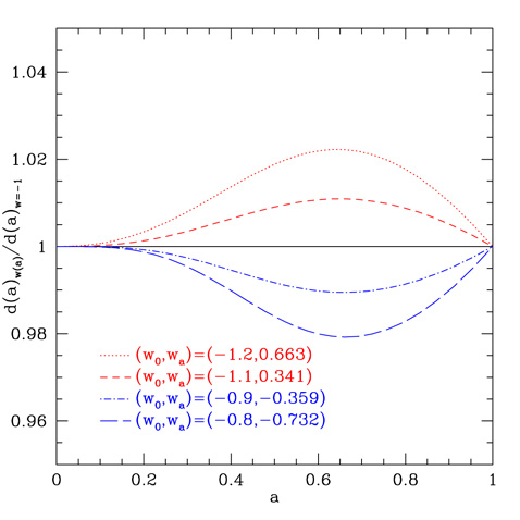
Figure 15. Matching the distance
to CMB last scattering between dark energy
models leads to convergence and crossover behaviors in other cosmological
quantities. The top left panel illustrates the convergence in the
distance-redshift relation, relative to the
|
|
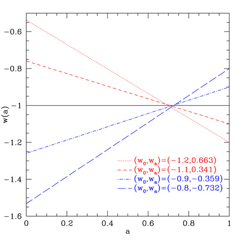
Matching the distance to last scattering imposes a relation between the
cosmological parameters, here shown as a family of
(w0, wa) models
holding other parameters fixed. The convergence in their distances
beginning at a
0.65 is associated with a similar convergence
in the fractional dark energy density, and a matching in
w(z) at a
0.7. Note that even
models with substantial time variation, wa
1, are forced to have
w(z
0.4) = -1, i.e. look like the cosmological constant. This is dictated by
the innate cosmological dependences of distance and is robust to
different parameter choices; see
[135]
for more details. (Note the matching in
 DE(a)
forced at a
0.5 has implications for the linear growth
factor and nonlinear power spectrum, as explored in
[144].)
DE(a)
forced at a
0.5 has implications for the linear growth
factor and nonlinear power spectrum, as explored in
[144].)
To see beyond the mirage of
, or test its
reality, requires measurements capable of directly probing the time
variation with significant sensitivity (hence extending out to z
1.7 as shown in
Section 3.1). Current and near term
experiments that may show w
-1 to a few percent
can induce a false sense of security
in . In
particular, the situation is exacerbated by the pivot
or decorrelation redshift (where the equation of state is measured most
precisely) of such experiments probing to z
1 being close to
the matching redshift imposed on w(z); so, given CMB data
consistent with ,
such experiments will measure w=-1 with great
precision, but possibly quite inaccurately. See
Figure 16
for a simulation of the possible data interpretation in terms of the
mirage of from an
experiment capable of achieving 1% minimum uncertainty on w
(i.e. w(zpivot)). Clearly, the time
variation wa is the important physical quantity
allowing us to see through the mirage, and the key science requirement
for next generation experiments.
 |
Figure 16. If CMB data are consistent with
|
Turning from theory to data analysis, another source of systematics that can lead to improper cosmological conclusions are heterogeneous data sets. This even holds with data all for a single cosmological probe, e.g. distances. Piecing together distances measured with different instruments under different conditions or from different source samples opens the possibilities of miscalibrations, or offsets, between the data.
While certainly an issue when combining, say, supernova distances with
baryon acoustic oscillation distances, or gravitational wave siren
distances, we illustrate the implications even for heterogeneous
supernova samples. An offset between the magnitude calibrations can
have drastic effects on cosmological estimation (see, e.g.,
[145]).
For example, very low redshift (z < 0.1) supernovae
are generally observed with very different telescopes and surveys than
higher redshift (z > 0.1) ones.
Since the distances in the necessary high redshift (z
1-1.7) sample
require near infrared observations from space then the crosscalibration
with the local sample (which requires very wide fields and more rapid
exposures) requires care. The situation is exacerbated if the space sample
does not extend down to near z
0.1-0.3 and a third
data set intervenes. This gives a second crosscalibration needed to high
accuracy.
Figure 17 demonstrates the impact on cosmology,
with the
magnitude offset leading to bias in parameter estimation. If there is
only a local distance set and a homogeneous space set extending from low
to high redshift, with crosscalibration at the 0.01 mag level, then the
biases take on the values at the left axis of the plot: a small fraction
of the statistical dispersion. However, with an intermediate data set,
the additional heterogeneity from matching at some further redshift
zmatch (with the systematic taken
to be at the 0.02 mag level to match a ground based, non-spectroscopic
experiment to a space based spectroscopic experiment) runs the risk of
bias in at least one parameter by of order
1 . Thus cosmological
accuracy advocates as homogeneous a data set as possible, ideally from
a single survey.
. Thus cosmological
accuracy advocates as homogeneous a data set as possible, ideally from
a single survey.
 |
Figure 17. Heterogeneous datasets open
issues of imperfect crosscalibration, modeled here as magnitude offsets
|
Similar heterogeneity and bias can occur in baryon acoustic oscillation surveys mapping the expansion when the selection function of galaxies varies with redshift. If the power spectrum shifts between samples, due for example to different galaxy-matter bias factors between types of galaxies or over redshift, then calibration offsets in the acoustic scale lead to biases in the cosmological parameters. Again, innate cosmology informs survey design, quantitatively determining that a homogeneous data set over the redshift range is advantageous.
Miscalibration involving the basic standard, i.e. candle luminosity or
ruler scale, has a pernicious effect biasing the expansion history mapping.
This time we illustrate the point with baryon acoustic oscillations. If
the sound horizon s is improperly calibrated, with an offset
 s
(for example through early dark energy effects in the prerecombination
epoch
[146,
147]),
then every baryon acoustic oscillation scale measurement
s
(for example through early dark energy effects in the prerecombination
epoch
[146,
147]),
then every baryon acoustic oscillation scale measurement
 (z)
= d(z) / s
and
(z)
= d(z) / s
and  (z)
= sH(z) will be miscalibrated.
Due to the redshift dependence of the untilded quantities, the offset will
vary with redshift, looking like an evolution that can be confused with a
cosmological model biased from the reality.
(z)
= sH(z) will be miscalibrated.
Due to the redshift dependence of the untilded quantities, the offset will
vary with redshift, looking like an evolution that can be confused with a
cosmological model biased from the reality.
To avoid this pitfall, analysis must include a calibration parameter for
the sound horizon (since CMB data does not uniquely determine it
[148,
147]),
in exact analogy to the absolute luminosity
calibration parameter  required for supernovae. That is, the standard ruler must be
standardized; assuming standard CDM prerecombination for the
early expansion history blinds the analysis to the risk of biased
cosmology results.
required for supernovae. That is, the standard ruler must be
standardized; assuming standard CDM prerecombination for the
early expansion history blinds the analysis to the risk of biased
cosmology results.
The necessary presence of a standard ruler calibration parameter, call it
 , leads to an increase in the
w0 - wa contour area, and
equivalent decrease in the "figure of merit" defined by that area, by
a factor 2.3. Since we
do not know a priori whether the high redshift universe is conventional CDM
(e.g. negligible early dark energy or coupling),
neglecting for BAO is as
improper as neglecting
for supernova standard
candle calibration. (Without the need to fit for the low redshift
calibration , SN would enjoy
an improvement in "figure of merit" by a factor 1.9, similar to the 2.3
that BAO is given when neglecting the high redshift calibration
.)
, leads to an increase in the
w0 - wa contour area, and
equivalent decrease in the "figure of merit" defined by that area, by
a factor 2.3. Since we
do not know a priori whether the high redshift universe is conventional CDM
(e.g. negligible early dark energy or coupling),
neglecting for BAO is as
improper as neglecting
for supernova standard
candle calibration. (Without the need to fit for the low redshift
calibration , SN would enjoy
an improvement in "figure of merit" by a factor 1.9, similar to the 2.3
that BAO is given when neglecting the high redshift calibration
.)
For supernovae, in addition to the fundamental calibration of the absolute luminosity, experiments must tightly constrain any evolution in the luminosity [149]. This requires broadband flux data from soon after explosion to well into the decline phase, and spectral data over a wide frequency range. Variations in supernova properties that do not affect the corrected peak magnitude do not affect the cosmological determination.
Distance measurements from the cosmological inverse square law of flux must avoid threshold effects where only the brightest sources at a given distance can be detected, known as Malmquist bias. Suppose the most distant, and hence dimmest, sources were close to the detection threshold. We can treat this selection effect as a shift in the mean magnitude with a toy model,
 |
(22) |
Consider a data set of some 1000 supernovae from z=0-1, with the Malmquist bias setting in at z* = 0.8 (where ground based spectroscopy begins to get quite time intensive and many spectral features move into the near infrared). The bias in a cosmological parameter relative to its uncertainty is then
 |
(23) |
for p =
(m,
w0, wa). Thus, the Malmquist bias
must be limited to less
than 0.05 mag at z = 0.95 to prevent significant bias in the derived
cosmological model. In fact, this is not a problem for
a well designed supernova survey since the requirement of mapping out
the premaximum phase of the supernova ensures sensitivity to fluxes
at least two magnitudes below detection threshold.
In addition to the theory interpretation and data analysis systematics discussed in this section, recall the fundamental theory systematics of Section 4.4.3 and Table 2. We finish with a very brief mention of some other selected data and data analysis systematics issues of importance that are often underappreciated and that must be kept in mind for proper survey design and analysis.
combining the absolute
luminosity and Hubble constant in
the case of supernovae, is often referred to as a nuisance parameter
but its proper treatment is essential. Although in some χ2
formulas for the distance-redshift relation it is not written explicitly,
it is implicit and cannot be ignored. More subtle is the issue of analytic
marginalization over it - this must be used with great care
as the distribution of is
actually
non-Gaussian due to interaction with other supernovae peak magnitude
fitting quantities (such as the lightcurve width and color terms)
[44].
Further subtleties exist between marginalization and minimization in
a multidimensional fit space
[155,
152],
and most analysis from raw data to quoted parameters actually employs
minimization techniques.
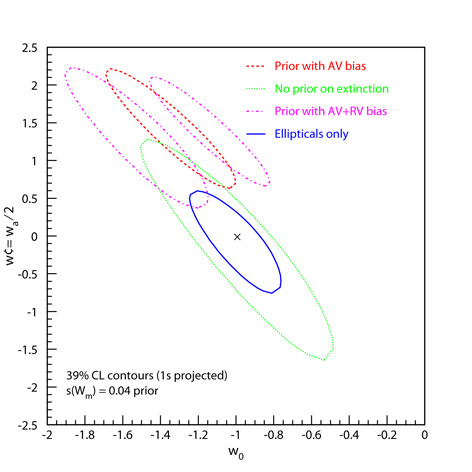 |
Figure 18. Assuming a prior on dust properties (AV and RV) in order to reduce extinction errors can cause systematic deviations in the magnitudes. These give strong biases to the equation of state, leading to a false impression of a transition from w < -1 to w > -1. To avoid this systematic, one can use samples with minimal extinction (elliptical galaxy hosted supernovae) or obtain precise multiwavelength data that allows for fitting the dust and color properties. Based on [157]. |
 m. One
scenario involves calibration between a local (z < 0.1)
spectroscopic set and a uniform survey extending from z
m. One
scenario involves calibration between a local (z < 0.1)
spectroscopic set and a uniform survey extending from z