VII. Production in the Early Universe

A. Review of Big Bang Cosmology

To understand how dark matter particles could have been created in the early universe, it is necessary to give a brief review of the standard model of cosmology. The standard model of cosmology, or the "Big Bang Theory" in more colloquial language, can be summed up in a single statement: the universe has expanded adiabatically from an initial hot and dense state and is isotropic and homogeneous on the largest scales. Isotropic here means that the universe looks the same in every direction and homogeneous that the universe is roughly the same at every point in space; the two points form the so-called cosmological principle which is the cornerstone of modern cosmology and states that "every comoving observer in the cosmic fluid has the same history" (our place in the universe is in no way special). The mathematical basis of the model is Einstein's general relativity and it is experimentally supported by three key observations: the expansion of the universe as measured by Edwin Hubble in the 1920s, the cosmic microwave background, and big bang nucleosynthesis.

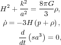
The Friedmann equations are the result of applying general relativity to a four dimension universe which is homogeneous and isotropic:

(7) (8) (9)

where H is the Hubble constant (which gives the expansion rate of the Universe and is not really a constant but changes in time), k is the four-dimensional curvature, G is Newton's gravitation constant, and p and are the pressure and energy density respectively of the matter and radiation present in the universe. a is called the scale-factor which is a function of time and gives the relative size of the universe (a is define to be 1 at present and 0 at the instant of the big bang), and s is the entropy density of the universe. The Friedmann equations are actually quite conceptually simple to understand. The first says that the expansion rate of the universe depends on the matter and energy present in it. The second is an expression of conservation of energy and the third is an expression of conservation of entropy per co-moving volume (a co-moving volume is a volume where expansions effects are removed; a non-evolving system would stay at constant density in co-moving coordinates even through the density is in fact decreasing due to the expansion of the universe).

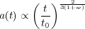
The expansion rate of the universe as a function of time can be determined by specifying the matter or energy content through an equation of state (which relates energy density to pressure). Using the equation of state = w p, where w is a constant one finds:

(10)

where t₀ represents the present time such that a(t₀)=1 as stated earlier. For non-relativistic matter where pressure is negligible, w = 0 and thus a t^2/3; and for radiation (and highly relativistic matter) w = 1/3 and thus a t^1/2. Although the real universe is a mixture of non-relativistic matter and radiation, the scale factor follows the dominant contribution; up until roughly 47,000 years after the big bang, the universe was dominated by radiation and hence the scale factor grows like t^1/2. Since heavy particles like dark matter were created before nucleosynthesis (which occurred minutes after the big bang), we shall treat the universe as radiation dominated when considering the production of dark matter.

B. Thermodynamics in the Early Universe

Particle reactions and production can be modeled in the early universe using the tools of thermodynamics and statistical mechanics. In the early universe one of the most important quantities to calculate is the reaction rate per particle:

(11)

where n is the number density of particles, is the cross section (the likelihood of interaction between the particles in question), and v is the relative velocity. As long as >> H(t) we can apply equilibrium thermodynamics (basically this measures if particles interact frequently enough or is the expansion of the universe so fast that particles never encounter each other). This allows us to describe a system macroscopically with various state variables: V (volume), T (temperature), E (energy), U (internal energy), H (enthalpy), S (entropy), etc. These variables are path independent; so long as two systems begin and end at the same value of a state variable, the change in that variable for both systems is the same. The most relevant quantity in the early universe is temperature. Since time and temperature are inversely correlated (t 1/T, i.e. the early universe is hotter), we can re-write the Hubble constant and reaction rates and cross sections in terms of temperature. The temperature will also tell us if enough thermal energy is available to create particles; for example, if the temperature of the universe is 10 GeV, sufficient thermal energy exists to create 500 MeV particles from pair production, but not 50 GeV particles.

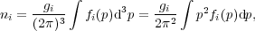
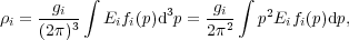
Statistical thermodynamics can be used to derive relations for the energy density, number density, and entropy density of particles in the early universe in equilibrium. To do so, Bose-Einstein statistics are used to describe distributions of bosons and Fermi-Dirac statistics are used to describe distributions of fermions. The main difference between the two arises from the Pauli exclusion principle which states that no two identical fermions can occupy the same quantum state at the same time. Bosons, on the other hand, can occupy the same quantum state at the same time. Hence there are small differences in the quantities we compute for bosons and fermions. To obtain the relevant statistical quantities, we begin with the distribution factor. The distribution factor f_i(p) for a particle species i is defined as

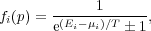(12)

where E_i = (m_i² + p²)^1/2, µ_i is the chemical potential of species i (energy associated with change in particle number), and the +1 case describes bosons and the -1 case fermions. (You might notice that the Boltzmann constant k is missing from the denominator of the exponential. To simplify things, cosmologists use a system of units where = k = c = 1.) The distribution factor can be used to determine ratios and fractions of particles at different energies, as well as the number and energy densities which are given by the integrals

(13)

and

(14)

where d³p = 4 p² dp and g_i is the number of degrees of freedom. The degrees of freedom are also called the statistical weights and basically account for the number of possible combinations of states of a particle. For example, consider quarks. Quarks have two possible spin states and three possible color states, and there are two quarks per generation. So, the total degrees of freedom for the quarks in the Standard Model are g_q = 2 × 3 × 2 = 12 with an addition g = 12 for the anti-quarks. Each fundamental type of particle (and associated anti-particle) has its own number of degrees of freedom, which enter into the calculations of number and energy densities. The known particles of the SM (plus the predicted Higgs boson) have a total of 118 degrees of freedom.

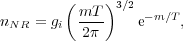
The integrals for number and energy densities can be solved explicitly in two limits: 1) the relativistic limit where m << T and 2) the non-relativistic limit where m >> T. For nonrelativistic particles where m >> T,

(15)

which is a Maxwell-Boltzmann distribution (no difference between fermions and bosons) and

(16)

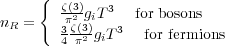
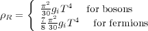
For relativistic particles, on the other hand, where m >> T,

(17)

and

(18)

where is the Riemann Zeta function. These results show that at any given time (or temperature) only relativistic particles contribute significantly to the total number and energy density; the number density of non-relativistic species are exponentially suppressed. As an example, knowing that the CMB photons have a temperature today of 2.73 K, we can use Eq. (17) to calculate n 410 photons/cm³.

C. Particle Production and Relic Density: The Boltzmann Equation

In the early universe, very energetic and massive particles were created and existed in thermal equilibrium (through mechanisms like pair production or collisions/interactions of other particles). In other words, the processes which converted heavy particles into lighter ones and vice versa occurred at the same rate. As the universe expanded and cooled, however, two things occurred: 1) lighter particles no longer had sufficient kinetic energy (thermal energy) to produce heavier particles through interactions and 2) the universe's expansion diluted the number of particles such that interactions did not occur as frequently or at all. At some point, the density of heavier particles or a particular particle species became too low to support frequent interactions and conditions for thermal equilibrium were violated; particles are said to "freeze-out" and their number density (no longer affected by interactions) remains constant. The exact moment or temperature of freeze-out can be calculated by equating the reaction rate, Eq. (11), with the Hubble (expansion) rate. The density of a specific particle at the time of freeze-out is known as the relic density for this particle since its abundance remains constant (see Fig. 5).

We know that a supersymmetric particle like the neutralino is a good dark matter candidate: it is electrically neutral, weakly interacting, and massive. It is also produced copiously in the early universe. But can a particle like the neutralino (or a generic WIMP) still exist in the present day universe with sufficient density to act as dark matter? To answer this question we will explore how precisely to compute relic densities.

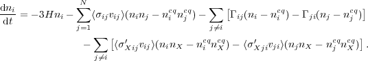
The Boltzmann equation gives an expression for the changing number density of a certain particle over time, dn / dt. To formulate the Boltzmann equation for a particle species, relevant processes must be understood and included. For supersymmetric particles, like the neutralino, there are four: 1) the expansion of the universe, 2) coannihilation, in which two SUSY particles annihilate with each other to create standard model particles, 3) decay of the particle in question, and 4) scattering off of the thermal background. Each of these processes then corresponds respectively to a term in the Boltzmann equation for dn_i / dt where there are N SUSY particles:

(19)

In the case of supersymmetry (which we will focus on for the rest of this section) the Boltzmann equation can be simplified by considering R-parity. If we also assume that the decay rate of SUSY particles is much faster than the age of the universe, then all SUSY particles present at the beginning of the universe have since decayed into neutralinos, the LSP. We can thus say that the abundance of neutralinos is the sum of the density of all SUSY particles (n = n_i +...+ n_N). Note, then, that when we take the sum in Eq. (19), the third and fourth terms cancel. This makes sense, because conversions and decays of SUSY particles do not affect the overall abundance of SUSY particles (and therefore neutralinos), and thus make no contribution to dn / dt. We are left with

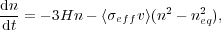(20)

where n is the number density of neutralinos, < _eff v > is the thermal average of the effective annihilation cross section _eff times the relative velocity v, and n_eq is the equilibrium number density of neutralinos. A quick note should be made about the thermal average < _eff v > and the added difficulty behind it. As thoroughly described by M. Schelke, coannihilations between the neutralinos and heavier SUSY particles can cause a change in the neutralino relic density of more than 1000%, and thus should not be left out of the calculation. [52] The thermal average is then not just the cross section times relative velocity of neutralino-neutralino annihilation, but of neutralino-SUSY particle annihilations as well; many different possible reactions must be considered based upon the mass differences between the neutralino and other SUSY particles.

By putting Eq. (20) in terms of Y = n / s and x = m / T where T is the temperature to simplify the calculations, we obtain the form

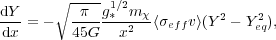(21)

where g_*^1/2 is a parameter which depends on the effective degrees of freedom. Eq. (21) can then be integrated from x = 0 to x₀ = m / T₀ to find Y₀ (which will be needed in Eq. (22) for the relic density). [62]

Fig. (5) (adapted from Kolb and Turner's excellent treatment of this topic [54]) plots an analytical approximation to the Boltzmann Equation and illustrates several key points. The y-axis is essentially (or at least proportional to) the relic density; the solid line is the equilibrium value and the dashed-line is the actual abundance. Notice that at freeze-out, the actual abundance leaves the equilibrium value and remains essentially constant; the equilbrium value, on other hand, continues to decrease so freeze-out is key to preserving high relic densities. Furthermore, the larger the annihilation cross section, < _a v >, the lower the relic density; this makes sense since the more readily a particle annihilates, the less likely it will exist in large numbers today. This has been paraphrased by many as "the weakest wins" meaning that particles with the smallest annihilation cross sections will have the largest relic densities.

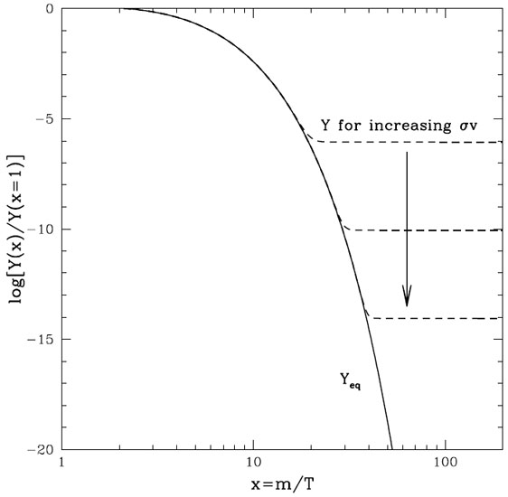Figure 5. The evolution of Y(x) / Y(x = 1) versus x = m / T where Y = n / s.

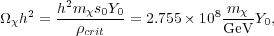
Using the value of Y₀ described above, the the relic density of neutralinos is given by

(22)

where m is the mass of the neutralino, s₀ is the entropy density today (which is dominated by the CMB photons since there are about 10¹⁰ photons per baryon in the universe), and Y₀ is the result of integrating the modified version of the Boltzmann equation. For a more thorough discussion of the Boltzmann equation and the relic density of neutralinos, consult M. Schelke and J. Edsjö and P. Gondolo. [52, 53]

Recall that the difference between the matter and baryon densities (as determined by WMAP) was h² = 0.11425 ± 0.00311. Can particle models of dark matter like SUSY or Kaluza-Klein theories produce dark matter in sufficient quantities to act as the bulk of the dark matter? The answer generically is yes. Although SUSY theories cannot predict a single dark matter relic density due to the inherent uncertainty in the input parameters, the Standard Model plus supersymmetry does produce a wide range of models some of which have the expected dark matter density. For example, MSSM models (the minimal supersymmetric standard model) yield dark matter relic densities from 10^-6 of the WMAP results to some which overclose the universe; neutralino masses for the models which give a correct relic abundance typically lie in the range 50-1000 GeV. A similar calculation can be performed for Kaluza-Klein dark matter in the Universal Extra Dimension scenario; Hooper and Profumo report that with the first excitation of the photon as the LKP a relic abundance can be obtained in the proper range of 0.095 < _dm < 0.129 for LKK masses between 850 and 900 GeV. [46]

To summarize, statistical thermodynamics allows us to model conditions in the early universe to predict relic abundances of dark matter particles like neutralinos. What is remarkable is that such models produce dark matter abundances consistent with the range provided by cosmological measurements. Theories like SUSY and Kaluza-Klein theories are so powerful, in particular, because such calculations (even given a wide range of uncertainty in several parameters) are possible. Armed with the required relic density of dark matter and the various models proposed by theorists, experiments can search for dark matter in specific areas of allowed parameter space. In the next section we will discuss the methods and progress of the various detection schemes and experiments.