


A special case of analyzing SEDs of extragalactic sources is the problem of redshift estimation, a topic that is usually refered to as photometric redshifts (hereafter photo-z). This problem is distinct from all other estimates of physical properties because independent and more precise measurements of the same property are available for large samples in the form of spectroscopic redshifts. The method can thus be tested extensively and even calibrated empirically. It is also one of the earliest forms of SED fitting, having been suggested as a manner to go beyond the limits of early spectroscopy (Baum 1957).
For a working definition,
Koo (1999)
suggests the following: "photometric
redshifts are those derived from only images or photometry with
spectral resolution  /
/
 20. This choice of 20 is intended to exclude redshifts derived from slit
and slitless spectra, narrow
band images, ramped-filter imager, Fabry-Perot images, Fourier transform
spectrometers, etc." This definition leaves room for a wide variety of
approaches that are actively being explored by members of the community.
While today most studies build on a set of magnitudes or colors, recently
other observables have been utilized with good success, e.g., in the
work by
Wray and Gunn (2008).
However, all methods depend on strong features
in the SEDs of the objects, such as the Balmer break or even PAH features
(Negrello et
al. 2009).
20. This choice of 20 is intended to exclude redshifts derived from slit
and slitless spectra, narrow
band images, ramped-filter imager, Fabry-Perot images, Fourier transform
spectrometers, etc." This definition leaves room for a wide variety of
approaches that are actively being explored by members of the community.
While today most studies build on a set of magnitudes or colors, recently
other observables have been utilized with good success, e.g., in the
work by
Wray and Gunn (2008).
However, all methods depend on strong features
in the SEDs of the objects, such as the Balmer break or even PAH features
(Negrello et
al. 2009).
Traditionally, photometric redshift estimation is broadly split into two areas: empirical methods and the template-fitting approach. Empirical methods use a subsample of the photometric survey with spectroscopically-measured redshifts as a `training set' for the redshift estimators. This subsample describes the redshift distribution in magnitude and colour space empirically and is used then to calibrate this relation. Template methods use libraries of either observed spectra of galaxies exterior to the survey or model SEDs (as described in Section 2). As these are full spectra, the templates can be shifted to any redshift and then convolved with the transmission curves of the filters used in the photometric survey to create the template set for the redshift estimators.
Both methods then use these training sets as bases for the redshift
estimating routines, which include
 2-fitting and
various machine learning algorithms (e.g. artificial neural
networks, ANNs). The most popular combinations are
2-fitting with
templates and machine learning with empirical models.
For a review of the ideas and history of both areas, see
Koo (1999).
2-fitting and
various machine learning algorithms (e.g. artificial neural
networks, ANNs). The most popular combinations are
2-fitting with
templates and machine learning with empirical models.
For a review of the ideas and history of both areas, see
Koo (1999).
The preference of one over the other is driven by the limitations of our understanding of the sources and the available observations. Template models are preferred when exploring new regimes since their extrapolation is trivial, if potentially incorrect. Empirical models are preferred when large training sets are available and great statistical precision is required. Here we review these techniques and estimators, concentrating predominantly on the template method which is closer to the idea of SED fitting as discussed in the previous section.
Early on, the first empirical methods proved extremely powerful despite their simplicity (see e.g. Connolly et al. 1995a, Brunner et al. 1997, Wang et al. 1998). This was partly due to their construction, which should provide both accurate redshifts and realistic estimations of the redshift uncertainties. Even low-order polynomial and piecewise linear fitting functions do a reasonable job when tuned to reproduce the redshifts of galaxies (see e.g. Connolly et al. 1995a). These early methods provided superior redshift estimates in comparison to template-fitting for a number of reasons. By design the training sets are real galaxies, and thus suffer no uncertainties of having accurate templates. Similarly as the galaxies are a subsample of the survey, the method intrinsically includes the effects of the filter bandpasses and flux calibrations
One of the main drawbacks of this method is that the redshift estimation is only accurate when the objects in the training set have the same observables as the sources in question. Thus this method becomes much more uncertain when used for objects at fainter magnitudes than the training set, as this may extrapolate the empirical calibrations in redshift or other properties. This also means that, in practice, every time a new catalogue is created, a corresponding training set needs to be compiled.
The other, connected, limitation is that the training set must be large enough that the necessary space in colours, magnitudes, galaxy types and redshifts is well covered. This is so that the calibrations and corresponding uncertainties are well known and only limited extrapolations beyond the observed locus in colour-magnitude space are necessary.
The simplest and earliest estimators were linear and polynomial fitting, where simple fits of the empirical training set in terms of colours and magnitudes with redshift were obtained (see e.g. Connolly et al. 1995a). These could then be matched to the full sample, giving directly the redshifts and their uncertainties for the galaxies. Since then further, more computational intensive algorithms, have been used, such as oblique decision tree classification, random forests, support vector machines, neural networks, Gaussian process regression, kernel regression and even many heuristic homebrew algorithms.
These algorithms all work on the idea of using the empirical training set to build up a full relationship between magnitudes and/or colours and the redshift. As each individual parameter (say the B - V colour) will have some spread with redshift, these give distributions or probabilistic values for the redshift, narrowed with each additional parameter. This process, in terms of artificial neural networks, is nicely described by Collister and Lahav (2004), who use this method in their publicly available photo-z code ANNz (described in the same paper). They also discuss the limitations and uncertainties that arise from this methodology.
Machine learning algorithms (of which neural networks is one) are one of the strengths of the empirical method. These methods are able to determine the magnitude/colour and redshift correlations to a surprising degree, can handle the increasingly large training sets (i.e. SDSS) and return strong probabilistic estimates (i.e. well constrained uncertainties, see figure 16) on the redshifts (see Ball et al. 2008a for a description of machine learning algorithms available and the strong photo-z constraints possible). In addition, machine learning algorithms are also able to handle the terascale datasets now available for photo-z determination rapidly, limited only by processor speed and algorithm efficiency (Ball et al. 2008b).
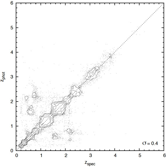 |
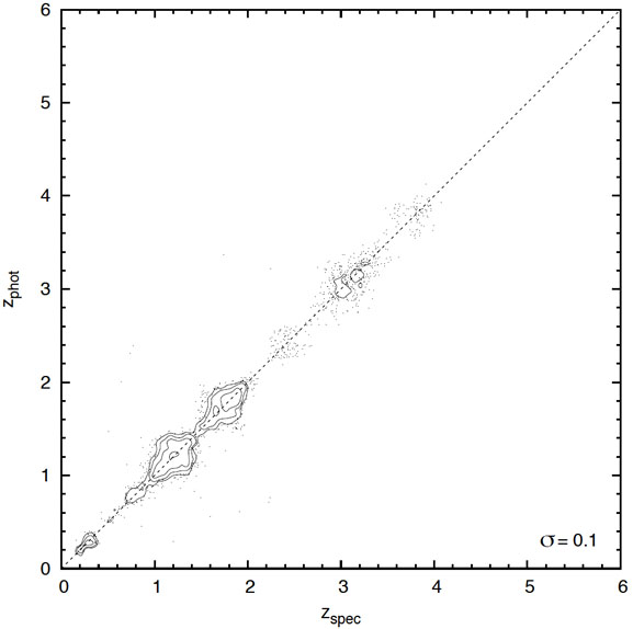 |
Figure 16. Improvement in quasar redshifts enabled by the Ball et al. (2008b) data mining techniques, shown as spectroscopic versus photometric redshift for the SDSS. Left: A reproduction, using their framework, a typical result prior to their work (e.g. Weinstein et al. 2004) Right: The result of using machine learning to assign probability density functions then taking the subset with a single peak in probability. Contours indicate the areal density of individual quasars (points) on the plot. Data from Ball et al. (2008b). [Courtesy N.Ball] |
|
The additional benefit of the empirical method with machine learning, now increasingly being used, is that the constraining inputs for the photo-zs are not limited to the galaxies SED. Suggested first by Koo (1999), properties such as the the bulge-to-total flux ratio (e.g. Sarajedini et al. 1999), surface brightness (e.g. Kurtz et al. 2007), petrosian radii (e.g. Firth et al. 2003), and concentration index (e.g. Collister and Lahav 2004) have all been used in association with the magnitudes and colours to constrain the redshift, some codes even bringing many of these together (e.g. Wray and Gunn 2008).
Unlike the empirical method, the template-based method is actually a form of SED fitting in the sense of this review (see e.g. Koo 1985, Lanzetta et al. 1996, Gwyn and Hartwick 1996, Pello et al. 1996, Sawicki et al. 1997). Put simply, this method involves building a library of observed (Coleman et al. 1980 is a commonly used set) and/or model templates (such as Bruzual and Charlot 2003) for many redshifts, and matching these to the observed SEDs to estimate the redshift. As the templates are "full" SEDs or spectra, extrapolation with the template fitting method is trivial, if potentially incorrect. Thus template models are preferred when exploring new regimes in a survey, or with new surveys without a complementary large spectroscopic calibration set. A major additional benefit of the template method, especially with the theoretical templates, is that obtaining additional information, besides the redshift, on the physical properties of the objects is a built-in part of the process (as discussed in section 4.1). Note though, that even purely empirical methods can predict some of these properties if a suitable training set is available (see e.g. Ball et al. 2004).
However, like empirical methods, template fitting suffers from several problems, the most important being mismatches between the templates and the galaxies of the survey. As discussed in section 2, model templates, while good, are not 100% accurate, and these template-galaxy colour mismatches can cause systematic errors in the redshift estimation. The model SEDs are also affected by modifiers that are not directly connected with the templates such as the contribution of emission lines, reddening due to dust, and also AGN, which require very different templates (see e.g. Polletta et al. 2007).
It is also important to make sure that the template set is complete, i.e. that the templates used represent all, or at least the majority, of the galaxies found in the survey (compare also Section 4.5.2). This is especially true when using empirical templates, as these are generally limited in number. Empirical templates are also often derived from local objects and may thus be intrinsically different from distant galaxies, which may be at different evolutionary stage. A large template set is also important to gauge problems with degeneracies, i.e. where the template library can give two different redshifts for the same input colours. Another potential disadvantage of template fitting methods comes from their sensitivity to many other measurements to about the percent level, e.g., the bandpass profiles and photometric calibrations of the survey.
For implementations of the template fitting, the method of
maximum likelihood is predominant. This usually involves the
comparison of the observed magnitudes with the magnitudes derived from
the templates at different redshifts, finding the match that minimizes
the 2 (compare
section 4.5). What is returned
is the best-fitting (minimum
2) redshift and
template (or
template+modifiers like dust attenuation). By itself this method does
not give uncertainties in redshift, returning only the best fit. For
estimations of the uncertainties in redshift, a typical process is to
propagate through the photometric uncertainties, to determine what is
the range of redshifts possible within these uncertainties. A good
description of the template-fitting, maximum likelihood method can be
found in the description of the publicly available photo-z code,
hyperz in
Bolzonella et
al. (2000).
As mentioned above, one of the issues of the templates is the possibility of template incompleteness, i.e. not having enough templates to describe the galaxies in the sample. Having too many galaxies in the template library on the other hand can lead to colour-redshift degeneracies. One way to overcome these issues is through Bayesian inference: the inclusion of our prior knowledge (see Section 4.5), such as the evolution of the upper age limit with redshift, or the expected shape of the redshift distributions, or the expected evolution of the galaxy type fractions. As described in Section 4.5, this has the added benefit of returning a probability distribution function, and hence an estimate of the uncertainties and degeneracies. In some respects, by expecting the template library to fit all observed galaxies in a survey, the template method itself is already Bayesian. Such methods are used in the BPZ code of Benítez (2000), who describes in this work the methodology of Bayesian inference with respect to photo-z, the use of priors and how this method is able to estimate the uncertainty of the resulting redshift.
It should be noted that, while public, prepackaged codes might provide reasonable estimates for certain types of sources, no analyses should proceed without cross-validation and diagnostic plots. There are common problems that appear in data sets and issues that need to be understood first, and worked around, if possible (see e.g. Mandelbaum et al. 2005 for a comparison of some public photo-z codes). Some further public photo-z codes include kphotoz (Blanton et al. 2003), ZEBRA (Feldmann et al. 2006) and Le Phare (Arnouts et al. 1999, Ilbert et al. 2006, Ilbert et al. 2009a).
5.2. Calibration and error budgets
Redshift errors are ultimately data-driven: they typically scale with 1+z given constant wavelength resolution of most filter sets; they also scale with photometric error in a transition regime between ~ 2% and ~ 20%. Smaller errors are often not exploited due to mismatches between data and model arising from data calibration and choice of templates, while large errors translate non-linearly into weak redshift constraints. If medium-band resolution is available, QSOs show strong emission lines and lead to deeper photo-z completeness for QSOs than for galaxies.
Photometric redshifts have limitations they share with spectroscopic ones, and some that are unique to them: as in spectroscopy, catastrophic outliers can result from the confusion of features, and completeness depends on SED type and magnitude. Two characteristic photo-z problems are mean biases in the redshift estimation and large and/or badly determined scatter in the redshift errors. Catastrophic outliers result from ambiguities in colour space: these are either apparent in the model and allow flagging objects as uncertain, or are not visible in the model but present in reality, in which case the large error is inevitable even for unflagged sources. Empirical models may be too small to show local ambiguities with large density ratios, and template models may lack some SEDs present in the real Universe.
Remedies to these issues include adding more discriminating data, improving the match between data and models as well as the model priors, and taking care with measuring the photometry and its errors correctly in the first place. Photo-z errors in broad-band surveys appear limited to a redshift resolution near 0.02 × (1 + z), a result of limited spectral resolution and intrinsic variety in spectral properties. Tracing features with higher resolution increases redshift accuracy all the way to actual spectroscopy. Future work among photo-z developers will likely focus on two areas: (i) Understanding the diversity of codes and refining their performance; and (ii) Describing photo-z issues quantitatively such that requirements on performance and scientific value can be translated into requirements for photometric data, for the properties of the models and for the output of the codes.
In general, template-based photo-z estimates depend sensitively on the set of templates in use. In particular, it has been found that better photo-z estimates can be achieved with an empirical set of templates (e.g. Coleman et al. 1980, Kinney et al. 1996) rather than using stellar population synthesis models (SPSs; e.g. Bruzual and Charlot 2003, Maraston 2005 see Section 2) directly. Yet the models are what are commonly used to compute stellar masses of galaxies. Since the use of these templates do not result in very good photometric redshifts, what is usually done, is to first derive photometric redshifts through empirical templates, and then estimate the stellar masses with the SSP templates. Obviously this is not self-consistent.
To investigate what causes the poorer photo-z estimates of synthetic templates, Oesch et al. (in prep.) used the photometric data in 11 bands of the COSMOS survey (Scoville et al. 2007), together with redshifts of the zCOSMOS follow-up (Lilly et al. 2007) and fit the data with SSP templates. In the resulting rest-frame residuals they identified a remarkable feature around 3500 Å, where the templates are too faint with respect to the photometric data, which can be seen in figure 17. The feature does not seem to be caused by nebular continuum or line emission, which they subsequently added to the original SSP templates. Additionally, all types of galaxies suffer from the same problem, independent of their star-formation rate, mass, age, or dust content.
 |
Figure 17. Rest-frame residuals
( |
Similar discrepancies have been found previously by Wild et al. (2007), Walcher et al. (2008), who found a ~ 0.1 mag offset in the Dn(4000) index. As this spectral break is one of the main features in the spectrum of any galaxy, it is likely that the poor photo-z performance of synthetic templates is caused by this discrepancy. The cause of the discrepancy has been identified as a lack of coverage in the synthetic stellar libraries used for the models. It will thus be remedied in the next version of GALAXEV (G. Bruzual, priv. comm.).
5.2.2. Spectroscopic Calibration of Photo-zs
One of the strong benefits of the template method is that any spectroscopic subsample of a survey can be used to check the template-determined photo-zs. This can also be done for the empirical methods, yet for this a very large spectroscopic sample is necessary such that it can be divided into a large enough training set and testing sets.
With the existence of a test spectroscopic sample, it is then possible to calibrate the template library, leading to a combined empirical-template method. This means to correct for errors in the photometric calibration or even the correction of the templates themselves for example to allow for the evolution of galaxies with a small library, or to account for inaccurate models (see section 2). Such calibration is typically an iterative process, in which the photometry and/or template SEDs are modified to minimize the dispersion in the resulting photometric redshifts.
The simplest kind of calibration involves adding small zero-point offsets to the photometry uniformly across the sample. This does not imply that the photometry is incorrectly calibrated (though in practice the absolute calibration may well have small errors in the zero-point), but rather that there is often a mismatch between the real SEDs of galaxies and the templates used to fit them. The calibration is meant to minimize those differences. Plotting color-color or color-redshift diagrams (figure 18) with the template SEDs overlaid will often indicate bulk offsets between the two.
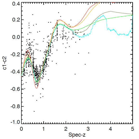 |
Figure 18. IRAC [3.6]-[4.5] color-redshift plot for a sample of GOODS galaxies. The solid curves show the change in colours with redshift of five different empirical template SEDs. [Courtesy M. Brodwin] |
A more instructive approach, however, is to compute the residuals
between the predicted magnitude of the best-fit template at the
spectroscopic redshift and the observed magnitude (for more details, see
Brodwin et
al. 2006a,
Brodwin et
al. 2006b).
These residuals can be plotted versus color or redshift for added
diagnostic power. In the example in Figure 19,
there appears to be an effective magnitude offset of
 0.3 mags in the
H-band.
0.3 mags in the
H-band.
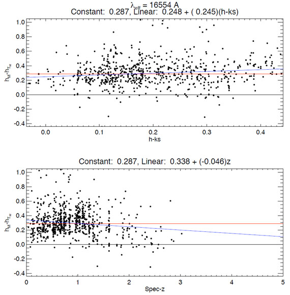 |
Figure 19. H-band residuals
vs. color and redshift in a sample of GOODS galaxies. An effective
offset of
|
Applying such effective zero-point adjustments in all bands in an iterative process minimizes the mismatch between the data and the templates, and hence minimizes the resultant photometric redshift dispersion, as shown in Fig. 20.
 |
Figure 20. Iterative improvement in photometric redshift estimation via this simple calibration technique. [Courtesy M. Brodwin] |
Such calibration phases are used in the works of Brodwin et al. (2006a) and as "template-optimization" in the codes ZEBRA (Feldmann et al. 2006) and Le Phare (Ilbert et al. 2006, Ilbert et al. 2009a) which use template fitting with Bayesian inferences and this calibration phase to give the most accurate photometric redshifts possible with the template approach.
With the most accurate photometric redshifts possible, the template-fitting can then be used to estimate physical properties such as stellar masses, star-formation rates, etc. (see section 6).
5.2.3. Signal-to-noise Effects
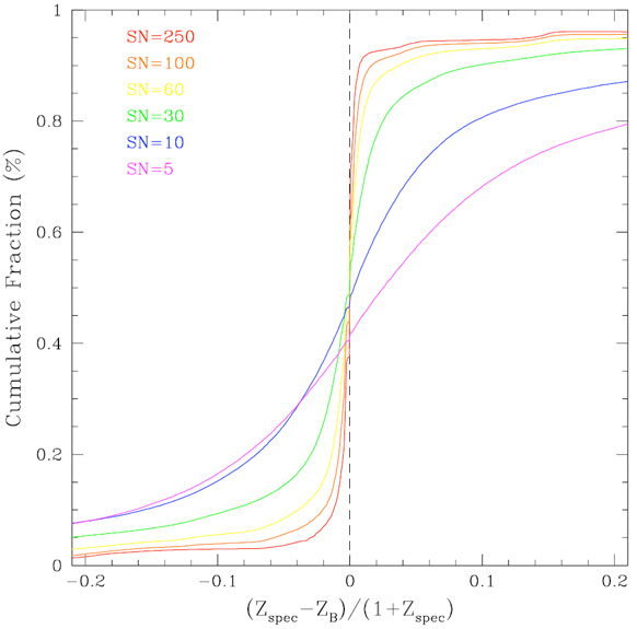
Margoniner and Wittman (2008) have specifically investigated the impact of photometric signal-to-noise (SN) on the precision of photometric redshifts in multi-band imaging surveys. Using simulations of galaxy surveys with redshift distributions (peaking at z ~ 0.6) that mimics what is expected for a deep (10-sigma R band = 24.5 magnitudes) imaging survey such as the Deep Lens Survey (Wittman et al. 2002) they investigate the effect of degrading the SN on the photometric redshifts determined by several publicly available codes (ANNz, BPZ, hyperz).
Figure 21 shows the results of one set of their
simulations for which they degraded the initially perfect photometry
to successively lower SN. In these unrealistic simulations all
galaxies have the same SN in all bands. The
figure shows the cumulative fraction of objects with
 z smaller than
a given value as a function of
z. The left
panel shows the cumulative fraction for all objects, while the right
panel shows galaxies for which the BPZ photo-z quality parameter,
ODDS > 0.9. The number of galaxies in
the right panel becomes successively smaller than the number in the left
as the signal-to-noise decreases (64% of SN = 250, and only 6.4% of SN = 10
objects have ODDS > 0.9), but the accuracy of photo-zs
is clearly better.
z smaller than
a given value as a function of
z. The left
panel shows the cumulative fraction for all objects, while the right
panel shows galaxies for which the BPZ photo-z quality parameter,
ODDS > 0.9. The number of galaxies in
the right panel becomes successively smaller than the number in the left
as the signal-to-noise decreases (64% of SN = 250, and only 6.4% of SN = 10
objects have ODDS > 0.9), but the accuracy of photo-zs
is clearly better.
 |
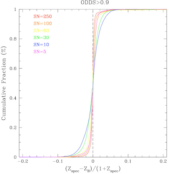 |
Figure 21. Cumulative fraction of
objects
with |
|
The results of this work show (1) the need to include realistic photometric errors when forecasting photo-zs performance; (2) that estimating photo-zs performance from higher SN spectroscopic objects will lead to overly optimistic results.
5.3. A unified framework The field of photometric redshifts and the estimation of other physical properties has been very pragmatic. Its development, since the first attempts, has been incremental in the sense that most studies focused on refining components but staying within the concepts of the original ideas of the two classes. Empirical and template-fitting approaches today follow very separate routes, with these classes of methods even use different sets of measurements. Only the semi-empirical approach of zero-point calibration comes close to linking the two approaches. However, a recent study by Budavári (2009a), tries to understand this separation and possibly bring these methods together by devising a unified framework for a rigorous solution based on first principles and Bayesian statistics.
This work starts with a minimal set of requirements: a training set with
some photometric observables x and spectroscopic
measurements  ,
and a query or test set with some potentially
different set of observables y. The link between these is
a model M that provides the mapping between x and
y, the probability density
p(x|y, M). This is more than
just the usual conversion formula between photometric systems because it
also incorporates the uncertainties.
,
and a query or test set with some potentially
different set of observables y. The link between these is
a model M that provides the mapping between x and
y, the probability density
p(x|y, M). This is more than
just the usual conversion formula between photometric systems because it
also incorporates the uncertainties.
The empirical relation of x -
is often
assumed to be a function. A better approach is to leave it general by
measuring the conditional density function.
The simplest way is to estimate the relation by the densities on the
training set as p(|x) =
p(,
x) / p(x). The final result is just a
convolution of the mapping and the measured relation:
p(|y, M) =
 dx
p(|x)p(x|y,
M). In figure 22 we show the results from
Budavári
(2009a),
where he plots the empirical relation (dotted blue line) and the final
probability density (solid red) for a handful of SDSS galaxies. The top
panels show intrinsically red galaxies, whose constraints are reasonably
tight out to the highest redshifts. Blue galaxies in the bottom panels
however get worse with the distance as expected.
dx
p(|x)p(x|y,
M). In figure 22 we show the results from
Budavári
(2009a),
where he plots the empirical relation (dotted blue line) and the final
probability density (solid red) for a handful of SDSS galaxies. The top
panels show intrinsically red galaxies, whose constraints are reasonably
tight out to the highest redshifts. Blue galaxies in the bottom panels
however get worse with the distance as expected.
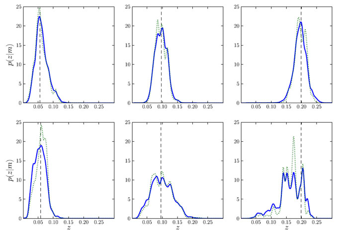 |
Figure 22. The probability density as a function of the redshift for early- and late-type galaxies (upper and lower panels, respectively) at different distances marked by the vertical dashed lines. For every object, the dotted line shows the empirical relation of p(z|x = mq), and the solid line illustrates the final result of p(z|y = mq,M) after properly folding in the photometric uncertainties via the mapping in the model (figure from Budavári 2009a). [Courtesy T. Budavari]. |
The aforementioned application follows a minimalist empirical approach but already goes beyond traditional methods. Template-fitting is in the other extreme of the framework where the training set is generated from the model using some grid. Without errors on the templates, the equations reduce to the usual maximum likelihood estimation that is currently used by most codes. A straight forward extension Budavári (2009a) suggests is to include more realistic errors for the templates. Similarly one can develop more sophisticated predictors that leverage existing training sets and spectrum models at the same time.
5.4. The State of Photometric Redshifts
Generally there is an overall agreement in most aspects of photometric redshift methodologies, and even technicalities. However there is a need for standardized quality measures and testing procedures. It is important to analyze to performance of each model spectrum as a function of the redshift. This is best done by plotting the difference of the observed magnitudes and template-based ones. These figure can pinpoint problems with the spectra and even zero-points. Intrinsically these are the quantities used inside the template-optimization procedures, e.g., in Budavári et al. (2000) and Feldmann et al. (2006).
In SED fitting, interpolation between templates is often used, which can be done linearly or logarithmically. The latter has the advantage of being independent of the normalization of the spectra. Yet, most codes appear to use linear interpolation without a careful normalization. This might explain some of the discrepancies among similar codes found by the Photo-Z Accuracy Testing (PHAT) project. 5
The determination of the quality of the estimates is also a crucial topic. There is need for different measures that can describe the scatter of the points without being dominated by outliers and that can estimate the fraction of catastrophic failures. It is also recommended to characterize the accuracy of the estimates by a robust M-scale instead of the RMS; a measure that is simple to calculate, yet, not sensitive to outliers. Another aspect of this is the study of selection criteria that is often neglected. Certain projects are not concerned with incomplete samples as long as the precision of the ones provided is good (e.g., weak lensing, Mandelbaum et al. 2005), while others, such as galaxy clustering, might require an unbiased selection. Therefore, it is perceived that studies using methods with any quality flags or quantities should provide details of their selection effects.
A common theme for future goals in most photometric redshift works appears to be more detailed probabilistic analyses, with the need for probability density functions. Priors used in most bayesian analyses seem to be generally accepted in the photo-z community. With such consensus amongst photometric redshifts obtained, the focus of work now is shifting from the estimation of "just" the redshifts to simultaneously constraining physical parameters and the redshift in a consistent way.
5 http://www.astro.caltech.edu/twiki_phat/bin/view/Main/WebHome Back.