3. ANGULAR CLUSTERING

The spatial distribution of galaxies can be measured either in two dimensions as projected onto the plane of the sky or in three dimensions using the redshift of each galaxy. As it can be observationally expensive to obtain spectra for large samples of (particularly faint) galaxies, redshift information is not always available for a given sample. One can then measure the two-dimensional projected angular correlation function (), defined as the probability above Poisson of finding two galaxies with an angular separation :

(5)

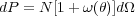
where N is the mean number of galaxies per steradian and d is the solid angle of a second galaxy at a separation from a randomly chosen galaxy.

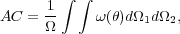
Measurements of () are known to be low by an additive factor known as the "integral constraint", which results from using the data sample itself (which often does not cover large areas of the sky) to estimate the mean galaxy density. This correction becomes important on angular scales comparable to the survey size; on much smaller scales it is negligible. One can either restrict measurements of the angular clustering to scales where the integral constraint is not important or estimate the amplitude of the integral constraint correction by doubly integrating an assumed power law form of () over the survey area, , using

(6)

where is the area subtended by the survey. In practice, this can be numerically estimated over the survey geometry using the random catalog itself (see Roche & Eales 1999 for details).

The projected angular two-point correlation function, (), can generally be fit with a power law,

(7)

where A is the clustering amplitude at a given scale (often 1^') and is the slope of the correlation function.

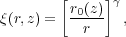
From measurements of () one can infer the three-dimensional spatial two-point correlation function, (r), if the redshift distribution of the sources is well known. The two-point correlation function, (r), is usually fit as a power law, (r) = (r / r₀)^-, where r₀ is the characteristic scale-length of the galaxy clustering, defined as the scale at which = 1. As the two-dimensional galaxy clustering seen in the plane of the sky is a projection of the three-dimensional clustering, () is directly related to its three-dimensional analog (r). For a given (r), one can predict the amplitude and slope of () using Limber's equation, effectively integrating (r) along the redshift direction (e.g. Peebles 1980). If one assumes (r) (and thus ()) to be a power law over the redshift range of interest, such that

(8)

then

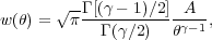(9)

where Γ is the usual gamma function. The amplitude factor, A, is given by

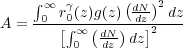(10)

where dN / dz is the number of galaxies per unit redshift interval and g(z) depends on and the cosmological model:

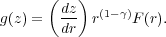(11)

Here F(r) is the curvature factor in the Robertson-Walker metric,

(12)

If the redshift distribution of sources, dN / dz, is well known, then the amplitude of () can be predicted for a given power law model of (r), such that measurements of () can be used to place constraints on the evolution of (r).

Interpreting angular clustering results can be difficult, however, as there is a degeneracy between the inherent clustering amplitude and the redshift distribution of the sources in the sample. For example, an observed weakly clustered signal projected on the plane of the sky could be due either to the galaxy population being intrinsically weakly clustered and projected over a relatively short distance along the line of sight, or it could result from an inherently strongly clustered distribution integrated over a long distance, which would wash out the signal. The uncertainty on the redshift distribution is therefore often the dominant error in analyses using angular clustering measurements. The assumed galaxy redshift distribution (dN / dz) has varied widely in different studies, such that similar observed angular clustering results have led to widely different conclusions. A further complication is that each sample usually spans a large range of redshifts and is magnitude-limited, such that the mean intrinsic luminosity of the galaxies is changing with redshift within a sample, which can hinder interpretation of the evolution of clustering measured in () studies.

Many of the first measurements of large scale structure were studies of angular clustering. One of the earliest determinations was the pioneering work of Peebles (1975) using photographic plates from the Lick survey (Fig. 1). They found () to be well fit by a power law with a slope of = -0.8. Later studies using CCDs were able to reach deeper magnitude limits and found that fainter galaxies had a lower clustering amplitude. One such study was conducted by Postman et al. (1998), who surveyed a contiguous 4° by 4° field to a depth of I_AB = 24 mag, reaching to z ~ 1. Later surveys that covered multiple fields on the sky found similar results. The lower clustering amplitude observed for galaxies with fainter apparent magnitudes can in principle be due either to clustering being a function of luminosity and/or a function of redshift. To disentangle this dependence, each author assumes a dN/dz distribution for galaxies as a function of apparent magnitude and then fits the observed () with different models of the redshift dependence of clustering. While many authors measure similar values of the dependence of () on apparent magnitude, due to differences in the assumed dN / dz distributions different conclusions are reached regarding the amount of luminosity and redshift dependence to galaxy clustering. Additionally, quoted error bars on the inferred values of r₀ generally include only Poisson and/or cosmic variance error estimates, while the dominant error is often the lack of knowledge of dN / dz for the particular sample in question.

Because of the sensitivity of the inferred value of r₀ on the redshift distribution of sources, it is preferable to measure the three dimensional correlation function. While it is much easier to interpret three dimensional clustering measurements, in cases where it is still not feasible to obtain redshifts for a large fraction of galaxies in the sample, angular clustering measurements are still employed. This is currently the case in particular with high redshift and/or very dusty, optically-obscured galaxy samples, such as sub-millimeter galaxies (e.g., Brodwin et al. 2008, Maddox et al. 2010). However, without knowledge of the redshift distribution of the sources, these measurements are hard to interpret.