


We saw in the previous section that the large-scale distribution of perturbations in the matter field has the potential to provide a wealth of cosmological information, as it encodes a number of different physical processes. When we observe the field by means of a galaxy survey, we see the evolved product of the linear field, as traced by galaxies. The differences between the galaxy field and the original linear matter perturbations can be understood using a number of simple models that help to explain how the build-up of structure leads to galaxy formation.
The simplest model for cosmological structure growth follows from
Birkhoff's theorem, which states that a spherically symmetric
gravitational field in empty space is static and is always described
by the Schwarzchild metric
(Birkhoff and
Langer 1923).
Thus, a homogeneous
sphere of uniform density with radius ap (subscript
p refers to
the perturbation) can itself be modelled using the same equations that
govern the evolution of the Universe, with scale factor a. From this
we can derive the linear growth rate (e.g.
Peebles 1980).
We assume that we have two spheres containing the same mass, one of
background density
 , and one
with density
p,
where
, and one
with density
p,
where
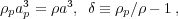 |
(16) |
giving, to first order in  ,
ap = a(1 -
/ 3). The
cosmological equation for both the spherical perturbation and the
background is
,
ap = a(1 -
/ 3). The
cosmological equation for both the spherical perturbation and the
background is
 |
(17) |
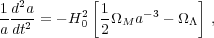
where a should be replaced by ap in the matter
density term for the perturbation, and we assume a
 CDM background
model. Using this equation for both spheres, and substituting in the
linear equation for as
a function of a and ap gives, to first order
CDM background
model. Using this equation for both spheres, and substituting in the
linear equation for as
a function of a and ap gives, to first order
 |
(18) |
where we have simplified this equation by including the evolution of
the matter and
densities with respect to the critical density,
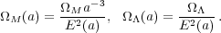 |
(19) |
E(a) was given in Eq. 13. This simple derivation, and
the solutions to this equation
(z)
∝ G(z), where G(z)
is the linear growth rate, show how large-scale densities grow within
the background Universe. More details of this derivation, and a
formula valid for general non-interacting Dark Energy models, are
given in
Percival (2005).
In the above subsection, we saw how the evolution of spherical perturbations follows that of mini-Universes, with different initial densities. A first-order solution was presented, giving the linear growth rate G(z). Going beyond the first order, the evolution of the perturbations can be followed further, until the effects of the assumption of homogeneity become apparent. Closed cosmological models, which are analogous to collapsed objects, start with sufficient density that the gravitational attraction overcomes Dark Energy leading to eventual collapse. Open cosmological models, which are analogous to under-dense regions, start with so little density that gravity cannot influence the initial expansion.
Fig. 1 shows the evolution of the perturbation scale for various initial conditions, and the link to the linear growth of perturbation scale. Given a low initial density, such as expected for a "void", the perturbation will expand more rapidly than the background, whereas more dense regions, such as large groups of galaxies, collapse. Within this simple model, collapse to a singularity is predicted; in practice the granulation of material leads to virialisation at a fixed radius.
 |
Figure 1. The evolution of the perturbation
scale factor ap, as a
function of the local density of the patch of universe under
consideration (solid lines). These were calculated for a flat
|
At any epoch, there is a critical initial density for collapse:
perturbations that are more dense have collapsed by the epoch of
interest, while less dense perturbations have not. For ease, the
critical density is usually extrapolated using linear theory to
present-day, and is called the linearly-extrapolated critical density
for collapse c.
c has a weak
dependence on cosmological model, and a review of methods to calculate
c is
given in, for example,
Percival (2005).
Given the weak dependence it is commonly approximated by its value for
an Einstein-de Sitter cosmological model
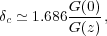 |
(20) |
where G(z) is the standard linear growth rate, which extrapolates the initial over-density to present day.
Taking the spherical model one step further it is possible to form a
"complete", although simplistic, model for structure growth as a
function of the mass of an object.
Press and Schechter
(1974)
introduced the
concept of smoothing the initial density field to determine the
relative abundances of perturbations with different mass. For a filter
of width R, corresponding to a mass scale M = 4/3
 R3 where
is the
average density of the Universe, smoothing the matter
field with power spectrum P(k) gives a further field with
spatial variance
R3 where
is the
average density of the Universe, smoothing the matter
field with power spectrum P(k) gives a further field with
spatial variance
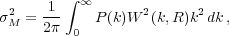 |
(21) |
where W(k, R) is the window function for the
smoothing. If a sharp
k-space filter is used then, around any spatial location, the smoothed
over-density forms a Brownian random walk in
, as a function of
filter radius (usually plotted as
 M2).
Comparing the
relative numbers of trajectories that have crossed the critical
density (as discussed in the previous section) at a mass greater than
that of interest (some may cross at high mass, but be below the
critical density at low mass, but still be counted as collapsed
objects), gives a distribution of haloes with mass (commonly called a
"mass function")
M2).
Comparing the
relative numbers of trajectories that have crossed the critical
density (as discussed in the previous section) at a mass greater than
that of interest (some may cross at high mass, but be below the
critical density at low mass, but still be counted as collapsed
objects), gives a distribution of haloes with mass (commonly called a
"mass function")
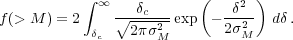 |
(22) |
Thus we have a complete model for structure formation: smoothing the fluctuations leads to the masses of collapsed objects, while the spherical perturbation model gives the epoch of collapse for those perturbations that are sufficiently dense. Comparing with numerical simulations reveals that, while this is a good model, it cannot accurately predict the measured redshift-dependent mass function, and fitting formulae to N-body simulations are the currently preferred way to model this (e.g. Sheth and Tormen 1999, Jenkins et al. 2001).
The above discussion only considered concentrations of mass, which are
commonly referred to as "haloes", whereas the most easily observed
extragalactic objects are galaxies. In general, a sample of galaxies
will form a Poisson sampling of some underlying field with over-density
g, but this
field may be different from the matter field, which has over-density
M. Here, a
subscript g refers to
galaxies, and M to the matter. This "bias" between fields encodes
the physics of galaxy formation, and may therefore be a general,
non-local, non-linear function. On large-scales we will now see that this
bias reduces to a local, linear function b
≡
g /
M.
The simplest model for large-scale galaxy bias is the peak-background
split model
(Bardeen et
al. 1986,
Cole and Kaiser
1989).
Here it is postulated that halo formation depends on the local density field
M. Large scale
density modes
l can
alter the local halo density n by
pushing pieces of the density field above a critical threshold,
leading to a change in the number density of haloes,
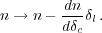 |
(23) |
To first order, the addition of the long wavelength mode leads to a bias,
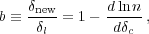 |
(24) |
where new is
the boosted over-density. Thus we see how
the shape of the mass function gives the large-scale (linear) bias of
haloes. On large scales we expect a linear relationship between the
large scale mode amplitudes and the change in number density, so the
shape of the galaxy and mass power spectra are the same.
Fig. 2 shows the result of the peak-background split model, giving the amplitude of clustering for haloes of different mass as a function of redshift. Higher mass haloes have stronger clustering as a result of the steeper mass function, which means that a small long-wavelength perturbation can have a disproportionate effect on the number density of haloes.
 |
Figure 2. The expected large-scale
clustering amplitude for haloes of
different mass as a function of scale, compared to the linear
growth rate. Clustering has been estimated using the
peak-background split model for a standard
|
On small scales, the peak-background split model no longer holds, and we must look to other models for the clustering of galaxies. One such model is the "halo" model (Seljak 2000, Peacock and Smith 2000, Cooray and Sheth 2002), which is a simple framework where galaxies trace halos on large scales, with bias determined by the distribution of halo masses within which the galaxies reside. On small scales, we expect galaxy clustering to be different from that of the halos, as pairs of galaxies inside single collapsed structures become important. The halo model simply combines these two scenarios into a full-scale model for galaxies.
 M =
0.25. The dashed lines
show the linear extrapolation of the initial perturbation
over-density. The dotted line shows the background
expansion. Within the simple spherical collapse model,
sufficiently over-dense regions collapse to singularities, while
under-dense regions expand forever. The relationship between the
linear growth of perturbations (discussed in
M =
0.25. The dashed lines
show the linear extrapolation of the initial perturbation
over-density. The dotted line shows the background
expansion. Within the simple spherical collapse model,
sufficiently over-dense regions collapse to singularities, while
under-dense regions expand forever. The relationship between the
linear growth of perturbations (discussed in