


In this section we explore some of the practical ideas and methods used to analyse a galaxy survey and make cosmological measurements. The clustering signal is a 3-dimensional signal, so ideally we wish to know the distribution of matter (or galaxies) in 3D. However, while the angular positions of galaxies are in general easy to measure, the radial distances are not so easy. In order to estimate distances to galaxies, large surveys typically use the spectrum of light emitted by galaxies, including absorption and emission lines and more general features, all resulting from the integrated stellar light. By comparing these features to rest-frame models, the redshifts of the galaxies can be estimated and, using the Hubble expansion rate, their distances.
It is possible to fit observed broad-band colours with templates or
training samples of emitted light profiles, and thus estimate galaxy
recession velocities. These "photometric redshifts" - redshifts
estimated from broad-band colours only - vary in quality between
galaxy samples. For example, they can have offsets from the true
redshifts with standard deviations of ~ 0.03(1 + z) for red galaxies
with strong 4000 Å breaks
(Ross et
al. 2011),
while more general populations can give estimates with
 z ~ 0.05(1 +
z). The level
of precision depends on the photometric quality of the data used, the
number of bands, etc. If spectra can be obtained for galaxies, then
absorption and emission lines can be used to estimate redshifts with
typical errors of ~ 0.001...0.0001(1 + z), allowing clustering along
the line-of-sight to be more accurately measured.
z ~ 0.05(1 +
z). The level
of precision depends on the photometric quality of the data used, the
number of bands, etc. If spectra can be obtained for galaxies, then
absorption and emission lines can be used to estimate redshifts with
typical errors of ~ 0.001...0.0001(1 + z), allowing clustering along
the line-of-sight to be more accurately measured.
4.1. Overview of galaxy surveys
Recent advances in galaxy surveys have largely been driven by new
instrumentation that enables multiple galaxy spectra to be obtained
simultaneously. Using these multi-object spectrographs (MOS), a number
of survey teams have created maps of many hundreds of thousands or
millions of galaxies. Key wide-field facilities include the
AA instrument on the Anglo-Australian Telescope, which has been used to
conduct the 2-degree Field Galaxy Redshift Survey (2dFGRS;
Colless et
al. 2003)
and Wigglez
(Drinkwater
et al. 2010)
surveys, and the Sloan Telescope, which has been used for the Sloan
Digital Sky Survey (SDSS;
York et al.
2000).
instrument on the Anglo-Australian Telescope, which has been used to
conduct the 2-degree Field Galaxy Redshift Survey (2dFGRS;
Colless et
al. 2003)
and Wigglez
(Drinkwater
et al. 2010)
surveys, and the Sloan Telescope, which has been used for the Sloan
Digital Sky Survey (SDSS;
York et al.
2000).
In following sections we will use results from the Baryon Oscillation Spectroscopic Survey (BOSS Dawson et al. 2013), part of the SDSS-III project (EEisenstein et al. 2011) to demonstrate possible measurements. BOSS is primarily a spectroscopic survey, which is designed to obtain spectra and derive redshifts from them for 1.2 million galaxies over an extragalactic footprint covering 10000 square degrees. 1000 spectra are simultaneously recovered in each observation, using aluminium plates with drilled holes to locate manually plugged optical fibres that feed a pair of double spectrographs. Each observation is performed in a series of 900-second exposures, integrating until a minimum signal-to-noise ratio is achieved for the faint galaxy targets. The resulting data set has high redshift completeness > 97 per cent over the full survey footprint.
As described in Section 1.1, we need to
translate from an
observed galaxy density to a dimensionless over-density. For a galaxy
survey, this means understanding where you could have observed
galaxies (called the survey mask), not just where galaxies were
observed. For current surveys, the mask can be split into independent
radial and angular components, where the angular component of the mask
includes the varying completeness and purity of observations and the
radial component depends on the galaxy selection criteria. For a
magnitude-limited catalogue, the radial distribution can be determined
by integrating under a model luminosity function
(ColeCole 2011),
while for a colour selected sample, a fit to the galaxy distribution
is usually performed
(Anderson et
al. 2012).
The mask is commonly
quantified by means of a random catalogue - a catalogue of spatial
positions that Poisson sample the expected density
 (see
Eq. 1), as outlined by the mask. This catalogue has the
same spatial selection function as the galaxies but no clustering.
(see
Eq. 1), as outlined by the mask. This catalogue has the
same spatial selection function as the galaxies but no clustering.
If the correct mask has been used, the estimate of
 g(x)
is unbiased, but has spatially varying noise, and we only have
estimates within the volume covered by the survey. In order to
optimally measure the amplitude of clustering, we need to apply
weights. If we assume that the galaxy field forms a Poisson sampling
of a field with expected power spectrum
g(x)
is unbiased, but has spatially varying noise, and we only have
estimates within the volume covered by the survey. In order to
optimally measure the amplitude of clustering, we need to apply
weights. If we assume that the galaxy field forms a Poisson sampling
of a field with expected power spectrum
 (k), then the
optimal weights to use are
(k), then the
optimal weights to use are
 |
(25) |
where  (x) is the
expected density of galaxies
(Feldman et
al. 1994).
The dependence on both
(x) and
(k)
in these weights balances the shot-noise and
sample-variance components of the measurement error. For multiple
samples of galaxies covering the same volume, but with different
expected clustering strengths (each sample is given a subscript i),
the optimal weights
(Percival et
al. 2004)
to apply are
(x) is the
expected density of galaxies
(Feldman et
al. 1994).
The dependence on both
(x) and
(k)
in these weights balances the shot-noise and
sample-variance components of the measurement error. For multiple
samples of galaxies covering the same volume, but with different
expected clustering strengths (each sample is given a subscript i),
the optimal weights
(Percival et
al. 2004)
to apply are
 |
(26) |
These weights provide the same balance between shot-noise and sample variance as Eq. 25, but now also balance this against the clustering strength of each sample. For example, galaxies with high clustering strength are up-weighted as these contain higher signal-to-noise. These weighting schemes assume that galaxies Poisson sample the underlying matter field, but this is only an approximation. In fact, galaxies live in matter haloes, and haloes do not Poisson sample the mass in the Universe: on large-scales the matter has a distribution with sub-Poisson variance. Thus applying a weighting based on the mass of the haloes within which the galaxies reside can reduce the shot noise in surveys (Seljak et al. 2009).
4.3. Measuring the power spectrum
If we only wish to measure the isotropically averaged power spectrum, then it is possible to simply measure this directly from a Fourier transform of the over-density field (Feldman et al. 1994). Suppose that we have a galaxy catalogue with density ng(x), and a random catalogue describing the mask with density nr(x) containing α times as many objects. Following Feldman et al. (1994), we start from the un-normalised over-density field
 |
(27) |
Taking the Fourier transform of this field, and calculating the power gives
 |
(28) |
where G(k) is the Fourier transform of the window function, defined by
 |
(29) |
and the final term in Eq. 28 gives the shot noise. We see that the effect of the survey mask, which is multiplicative in real-space (think of seeing the Universe through a window only revealing the patch observed), becomes a convolution in Fourier-space. There is a shot noise contribution on all scales, which can be subtracted from the power spectrum estimates, although it still contributes to the error. The fact that we have to estimate the mean density of galaxies from the sample itself means that the k = 0 mode is artificially set to zero, equivalent to subtracting a single Dirac delta function from the centre of the un-convolved power. The equivalent correction for correlation function estimates is commonly know as the "Integral constraint"
The comoving power spectrum, as measured from the Data Release 9 (DR9) BOSS data, using the Feldman et al. (1994) technique is shown in Fig. 3. The inset shows the ratio of the measured power to a smooth fit, isolating the signature of baryons (see Section 2.3), which is clearly visible (Anderson et al. 2012).
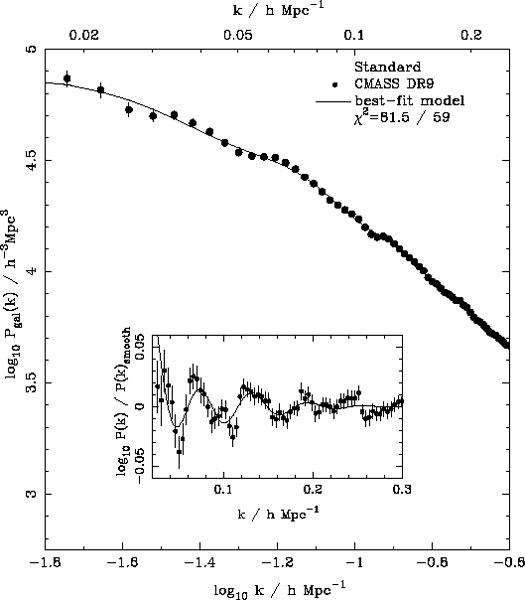 |
Figure 3. The spherically averaged BOSS DR9
power spectrum for the CMASS galaxy sample (solid circles with
1 |
We cannot easily measure the anisotropic power spectrum as a function of µ (see Section 1.5) using Fourier methods because the line-of-sight varies across a survey, and does not line-up with a Cartesian grid. Thus, to measure the anisotropic power spectrum, one either needs to manually perform the transform, so a different line-of-sight can be used for each galaxy pair (Yamamoto et al. 2006), or decompose into a basis that is itself separable along and across the spatially varying line-of-sight (e.g. Heavens and Taylor 1995). As surveys increase in size and statistical errors reduce, methods such as these will become increasingly important.
4.4. Measuring the correlation function
In order to estimate the correlation function, we can directly make
use of the idea of "throwing down sticks" described in
Section 1.2. Suppose that the mask is
quantified by a random catalogue as in Section 4.3,
then we can form an estimate of the correlation function

 |
(30) |
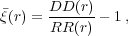
where DD(r) is the number of galaxy-galaxy pairs within a bin with centre r normalised to the maximum possible number of galaxy-galaxy pairs (ie. for n galaxies the maximum number of distinct pairs is n(n - 1) / 2). RR(r) is the normalised number of random-random pairs, and we can similarly define DR(r) as the normalised number of galaxy-random pairs.
This estimate of
 (r) is
biased and we find that
(r) is
biased and we find that
 |
(31) |
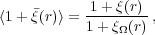
where (r) is the mean of the two-point
correlation function over the mask
(Landy and Szalay
1993):
this corrects for the fact
that the true mean density of galaxies
(r) is estimated
from the sample itself, normalising the total number of pairs. For
small samples, the factor [1 +
(r)], called
the "integral
constraint", limits the information that can be extracted from
(r)
- in the limit where we only observe pairs of a single
separation,
≃ , and
(r)
contains no information.
Because the galaxy and random catalogues are uncorrelated, <DR(r)> = < RR(r)>, and we can consider a number of alternatives to Eq. 30. In particular
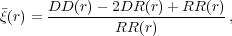 |
(32) |
has been shown to have good statistical properties (Landy and Szalay 1993), although Eq. 31 still holds for this estimator (ie. it still "suffers" from the integral constraint). Pair counting methods can be trivially extended to bin pairs in separation and angle to the line-of-sight, giving estimates of the anisotropic correlation function. It is also possible to directly integrate over µ, weighted by a Legendre polynomial to give estimates of the multipoles, or by top-hat windows in µ (called "Wedges"; Kazin et al. 2012). These moments of the correlation function provide a mechanism to compress the anisotropic correlation function while still retaining the majority of the available information.
An example correlation function, calculated from the BOSS DR9 CMASS
sample
(Anderson et
al. 2012)
is given in Fig. 4. The
BAO "bump" caused by the physics described in
Section 2.3 is clearly visible. On
large scales, the correlation function reduces in amplitude (note that
r2
is
plotted, enhancing the appearance of the large-scale noise), showing
that the galaxies are evenly distributed. In fact, conservation of
pair number means that the correlation function changes sign on very
large scales.
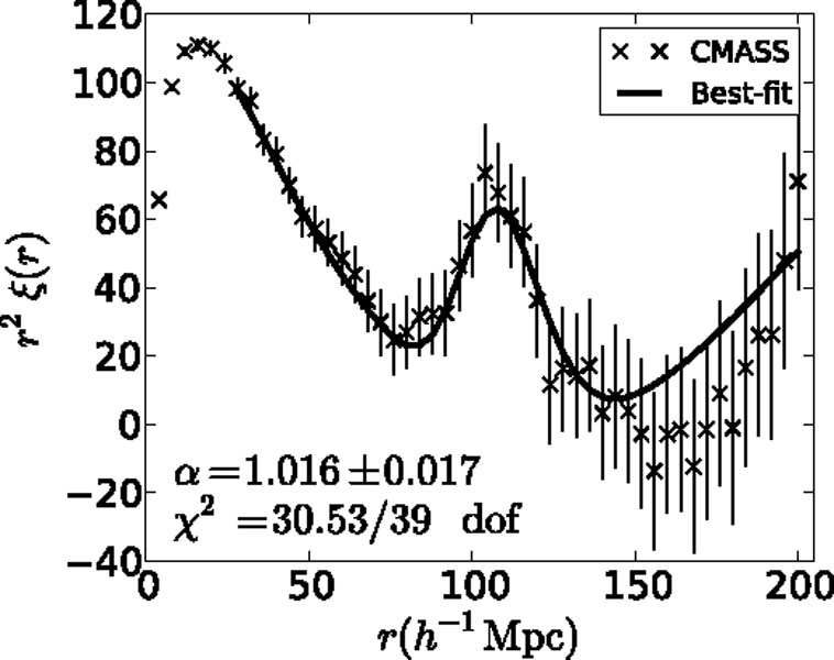 |
Figure 4. The spherically averaged BOSS DR9
correlation function for the CMASS galaxy sample (solid circles with
1 |
4.5. Reconstructing the linear density
In an evolved density field, pairs of over-densities initially separated by the BAO scale are subject to bulk motions that "smear" the initial pair separations. The matter flows and peculiar velocities act on intermediate scales (~ 20 Mpc h-1), and therefore suppress small-scale oscillations in the matter power spectrum and smooth the BAO feature in the correlation function (Eisenstein et al. 2007b, Crocce and Scoccimarro 2008, Matsubara 2008b, Matsubara 2008a). As galaxies trace the matter density field, the BAO in galaxy surveys are also damped. Eisenstein et al. (2007a) uggested that this smoothing can be reversed, in effect using the phase information within the density field to reconstruct linear behaviour. Although not a new idea (e.g. Peebles 1989, Peebles 1990, Nusser and Dekel 1992, Gramann 1993), the dramatic effect on BAO recovery had not been previously realised, and the majority of the benefit was shown to be recovered from a simple reconstruction prescription.
"Reconstruction" has been used to sharpen the BAO feature and improve distance constraints on mock data (Padmanabhan and White 2009, Noh et al. 2009, SSeo et al. 2010, Mehta et al. 2011), and was recently applied to the SDSS-II Luminous Red Galaxy (LRG) sample (Padmanabhan et al. 2012). The reconstruction was particularly effective in this case, providing a 1.9 per cent distance measurement at z = 0.35, decreasing the error by a factor of 1.7 compared with the pre-reconstruction measurement. On the BOSS DR9 CMASS sample, however, reconstruction was not as effective, and did not significantly reduce the error on the BAO scale measurement. Anderson et al. (2012) showed, using mock catalogues, that this is expected, and that the effectiveness of reconstruction varies across mocks. The average effect of reconstruction on the BOSS DR9 CMASS mocks is shown in Fig. 5.
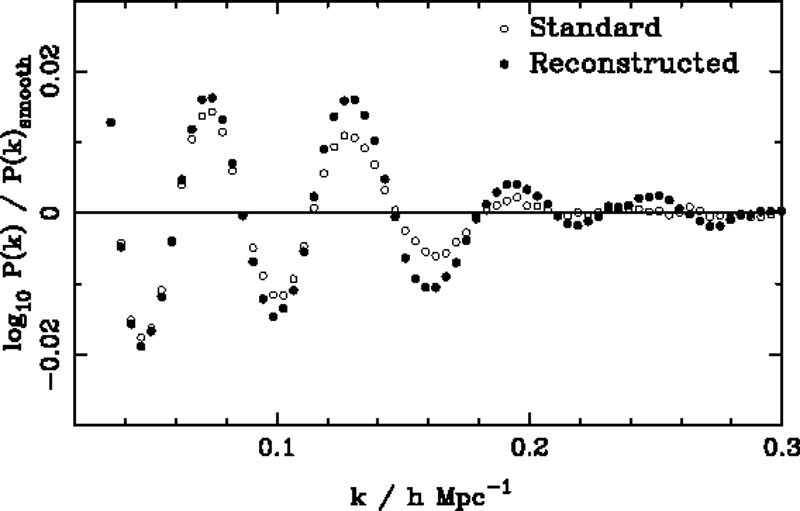 |
Figure 5. The ratio between recovered power spectrum and smooth fit for the 600 BOSS DR9 CMASS catalogues, before and after applying a simple reconstruction algorithm. We see that, on average, reconstruction acts to improve the BAO signal on small scales. Plot from Anderson et al. (2012). |
Light from distant quasars passes through intervening clouds of gas that absorb ultraviolet light predominantly at the wavelength of the Lyman alpha transition in neutral hydrogen (122 nm). The absorbing clouds are all at lower redshift than the quasar, so absorption lines are on the shorter wavelength side of the quasar emission line. Thus, if we divide the quasar spectrum by the expected continuum for each quasar, we are left with a 1D absorber over-density profile, which can be used to estimate the matter over-density field along the line-of-sight in much the same way that galaxies can be used directly (in fact the link between absorber density and matter density is more complicated than between galaxies and the mass). The great thing about using the Ly-α forest is that a single spectrum gives information about multiple structures along the line of sight, and thus this method provides a highly efficient use of telescopes. Using quasars with z > 2.15, the BOSS has made BAO measurements using Lyman α forest in quasar spectra, extending BAO measurements into the redshift range 2 < z < 3.5 (Busca et al. 2013, Slosar et al. 2013, Kirkby et al. 2013).