


In section 4 we discussed the cosmological 21 cmsignal and showed that it is expected to be on the order of ≈ 10 mK. However, the detectable signal in the frequency range that corresponds to the epoch of reionization is composed of a number of components each with its own physical origin and statistical properties. These components are: (1) the 21 cm signal coming from the high redshift Universe. (2) galactic and extra-galactic foregrounds, (3) ionospheric influences, (4) telescope response effects (5) Radio frequency interference (RFI) [146, 147] and (6) thermal noise (see Figure 2). Obviously, the challenge of the experiments in the low frequency regime is to distill the cosmological signal out of this complicated mixture of influences. This will depend crucially on the ability to calibrate the data very accurately so as to correct for the ever changing ionospheric effects and variation of the instrument response with time.
Currently, there are two types of redshifted 21 cm experiments that are
attempting to observe the EoR. The first type are experiments that
measure the global (mean) radio signal at the frequency range of
 = [100-200] MHz averaged over
the whole sky (hemisphere) as a
function of frequency. In this radio signal the 21 cm radiation
from the EoR is hidden. The expected measurement should show an increase
of the intensity at higher redshifts due to the increase in the neutral
fraction of H I. In particular, if the reionization
process occurred rapidly such a measurement should exhibit a step-like
jump in the mean brightness temperature at the redshift of reionization
zi (in this case zi is well defined).
This type of measurement is cheap and relatively easy to
perform. However, given the amount of foreground contamination,
especially from our Galaxy, radio frequency interference (RFI), noise
and calibration errors as well as the limited amount of information
contained in the data (mean intensity as a function of redshift), such
experiments are in reality very hard to perform. One
of those experiments, EDGES
[28],
has recently reported a lower limit on the duration of the reionization
process to be
= [100-200] MHz averaged over
the whole sky (hemisphere) as a
function of frequency. In this radio signal the 21 cm radiation
from the EoR is hidden. The expected measurement should show an increase
of the intensity at higher redshifts due to the increase in the neutral
fraction of H I. In particular, if the reionization
process occurred rapidly such a measurement should exhibit a step-like
jump in the mean brightness temperature at the redshift of reionization
zi (in this case zi is well defined).
This type of measurement is cheap and relatively easy to
perform. However, given the amount of foreground contamination,
especially from our Galaxy, radio frequency interference (RFI), noise
and calibration errors as well as the limited amount of information
contained in the data (mean intensity as a function of redshift), such
experiments are in reality very hard to perform. One
of those experiments, EDGES
[28],
has recently reported a lower limit on the duration of the reionization
process to be
 z > 0.06,
thus providing a very weak constraint on
reionization as most realistic simulations predict that
this process occurs over a much larger span of redshift
[27].
z > 0.06,
thus providing a very weak constraint on
reionization as most realistic simulations predict that
this process occurs over a much larger span of redshift
[27].
The second type of experiment is interferometric experiments carried out in the frequency range of ≈ 100-200 MHz, corresponding to a redshift range of ≈ 6-12. This type of experiment is considered more promising. The main reason for this is that these experiments allow better control of what is being measured and contain a huge amount of information so as to allow a much more accurate calibration of the instrument. Furthermore, radio interferometers are more diverse instruments that can be used to study many scientific topics besides the EoR, which makes them appealing for a much wider community. Having said that, however, one should note that the cost involved in building and running such facilities is much higher than for the global signal experiments.
 |
Figure 18. Left hand panel: A sketch
showing the basic principle of radio interferometry, the delay time
|
5.1. Radio Interferometry and the Calibration Problem
Interferometers measure the spatial correlation of the electric field
vector emanating from a distant source in the sky,
E(R,t), located at position R and
measured at time t. The sketch presented in the left hand panel of
Figure 18 shows the basic principle of
interferometry. The two stations (dishes) receive a wavefront from a
distant source and the receivers are timed to account for the difference
in the pathway to the two stations which obviously depends on the source
location on the sky. The signals measured
at the two stations, taken with the appropriate time difference
t, are then
cross-correlated (see for example
[200,
207]).
The measured spatial correlation of the electric field between two interferometric elements (stations) i and j is called the "visibility" and is approximately given by [200, 207]:
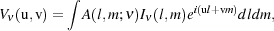 |
(23) |
where A is the normalized station response pattern and
I is the
observed intensity at frequency
.
The coordinates l and m are the projections (direction
cosines) of the source in terms of the baseline
in units of wavelength. As a side note, here we ignore the effect
of the Earth's curvature, the so called w-projection. From this equation
it is clear that the observed visibility is basically the Fourier
transform of the intensity measured at the coordinates u and v. Notice
that coordinates u and v depend on the baseline and its direction
relative to the source position (see the right hand panel of
Figure 18).
Therefore, the coordinates u and v produced by a given baseline vary
with time due to Earth's rotation and will create an arc in the uv plane
that completes half of the drawn track after 12 hours
as seen in the right hand panel of Figure 18.
The other half is produced due the fact that the intensity is a real
function. The width of the uv-track is set by the size of
the station, such that large stations produce thick tracks. I will
discuss the issue of uv coverage in more detail below.
One also should note that the coordinates u and v are a function
of wavelength, namely their value will change as a function of
frequency, which one has to take into account
when combining or comparing results from different frequencies.
In the interferometric visibilities there always exist errors introduced by the sky, the atmosphere (e.g. troposphere and ionosphere), the instrument (e.g. beam-shape, frequency response, receiver gains etc.) and by Radio Frequency Interference (RFI). The process of estimating and reducing the errors in these measurements is called calibration and is an essential step before understanding the measured data. Calibration normally involves knowing very well the position and intensities of the bright sources within and without the field of view of the radio telescope and using them to correct for the ionospheric and instrumental effects introduced into the data [76, 101, 155, 220]. This is similar to the adaptive optics techniques used in the optical regime except that here one needs to account for the variations in polarization of the radiation as well as in its total intensity.
Since most current instruments are composed of simple dipoles as their fundamental elements which have a polarized response (preferred x and y direction), the main danger in insufficient calibration lies in the possible leakage of polarized components into total intensity, thereby severely polluting the signal (see e.g., [94]). That is to say, since the cosmological signal is not expected to be polarized, if the polarized response of the instrument is not very well understood and taken into account it will mix some of the polarization that exists in the Galactic foregrounds (see subsection 5.5) with the cosmological signal and create a spurious signal that can not be distinguished from the cosmological signal. Hence, a very accurate calibration of these instruments is absolutely needed. Another issue one needs to deal with is that of the Radio Frequency interference, but we will not discuss it here and refer the reader instead to the papers by Offringa et. al. [146, 147].
5.2. Current and Future EoR Experiments
Currently, there are a number of new generation radio telescopes,
GMRT
2,
LOFAR
3,
MWA
4,
21CMA
5
and PAPER
6,
that plan to capture the lower redshift part of the
 Tb
evolution (z
Tb
evolution (z  12). Unfortunately, however, none of these experiments has enough
signal-to-noise to provide images of the EoR as it evolves with
redshift. Instead, they are all designed to detect the signal
statistically. In what follows I will focus on LOFAR more than the other
telescopes, simply because this is the instrument I know best, but the
general points I will make are applicable to the other telescopes as well.
12). Unfortunately, however, none of these experiments has enough
signal-to-noise to provide images of the EoR as it evolves with
redshift. Instead, they are all designed to detect the signal
statistically. In what follows I will focus on LOFAR more than the other
telescopes, simply because this is the instrument I know best, but the
general points I will make are applicable to the other telescopes as well.
The LOw Frequency ARray (LOFAR) is a European telescope built mostly in
the Netherlands and has two observational bands, a low band and a high
band covering the frequency range of 30-85 MHz and 115-230 MHz,
respectively. The high
band array is expected to be sensitive enough to measure the
redshifted 21 cm radiation coming from the neutral IGM within the
redshift range of z = 11.4 (115 MHz) to z = 6 (203 MHz), with a resolution
of 3-4 arcminutes and a typical field of view of ~ 120 square
degrees (with 5 beams) and a sensitivity on the order of 80 mK per
resolution element for a 1 MHz frequency bandwidth. At frequencies
below the FM band, probed by the low band array, the LOFAR sensitivity
drops significantly and the sky noise increases so dramatically (roughly
like ≈ -2.6) that
detection of H I signals at these frequencies is
beyond the reach of LOFAR
[77,
95,
103]
and all other current generation telescopes for that matter.
Figure 19 shows an artistic impression of the
LOFAR telescope and its spread over Europe (left hand panel). The right
hand panel shows the inner most center of the core located in the north
of the Netherlands and shows the two types of stations used in the array.
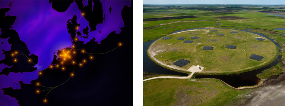 |
Figure 19. Left hand panel: An artist's impression of the layout of the LOFAR telescope over Western Europe. For the EoR, only the central part of the telescope is relevant. (courtesy of Peter Prijs). Right hand panel: The very central area of LOFAR. This circular area is know as the superterp and is the heart of the LOFAR core. The high-band array stations (covered in black blastic sheets) are clearly seen in this picture. In between one can also see the Low-Band Array antennas. |
In the future, SKA 7 [35] will significantly improve on the current instruments in two major ways. Firstly, it will have at least an order of magnitude higher signal-to-noise which will allow us to actually image the reionization process. It will also give us access to the Universe's dark ages up to redshifts as high as z ≈ 30 (assuming lowest frequency of about 50 MHz), hence, providing crucial information about cosmology which none of the current telescopes is able to probe. Thirdly, SKA will have a resolution better by a factor of few, at least, relative to the current telescopes [228]. These three advantages – sensitivity, resolution and frequency coverage – will not only improve on the understanding we gain with current telescopes but give the opportunity to address a host of fundamental issues that current telescopes will not be able to address at all. Here, I give a few examples: (1) due to the limited resolution and poor signal-to-noise of current telescopes, the nature of the ionizing sources is expected to remain poorly constrained; (2) the mixing between the astrophysical effects and the cosmological evolution is severe during the EoR but much less so during the dark ages, an epoch beyond the reach of the current generation of telescopes, but within SKA's reach; (3) at redshifts larger than 30, the 21 cm could potentially provide very strong constraints, potentially much more so than the CMB, on the primordial non-gaussianity of the cosmological density field, which is essential in order to distinguish between theories of the very early Universe (e.g., between different inflationary models).
5.3. Station configuration and uv coverage
In principle, Fourier space measurement and real space measurement are equivalent. However, this is only true if one has a perfect coverage of both spaces. In reality, each baseline will cover a certain line in the so called uv plane which needs to be convolved with the width of the track (see right hand panel of Figure 18). The combination of all the tracks of the array produces the uv coverage of the interferometer. The low frequency arrays must be configured so that they have a very good uv coverage. This is crucial to the calibration effort of the data where a filled uv plane is important for obtaining precise Local [143] and Global [184] Sky models (LSM/GSM; i.e. catalogues of the brightest, mostly compact, sources in and outside of the beam, i.e. local versus global). It is also crucial for the ability to accurately fit for the foregrounds [78, 95] and to the measurement of the EoR signal power spectrum [25, 77, 82, 176].
The uv coverage of an interferometric array depends on the layout of the stations (interferometric elements), their number and size as well as on the integration time, especially, when the number of stations is not large enough to have a good instantaneous uv coverage.
For a given total collecting area one can achieve a better uv coverage by having smaller elements (stations). For example LOFAR has chosen to have large stations resulting in about ≈ 103 baselines in the core area. Such a small number of baselines needs about 5-6 hours of integration time per field in order to fill the uv plane (using the Earth's rotation). In comparison, MWA which has roughly 1/3 of the total collecting area of LOFAR but chose to have smaller stations with about ≈ 105 baselines resulting in an almost instantaneous full uv coverage.
The decision on which strategy to follow has to do with a number of considerations that include the ability to store the raw visibilities, hence, allowing for a better calibration and an acceptable noise level for both the foreground extraction needs as well the power spectrum measurement (see the following sections; sec. 5.4 and sec. 5.5). A compromise between these issues as well the use of the telescopes for scientific projects other than the EoR is what drives the decision on the specific layout of the antennas.
In the low frequency regime the random component of the noise, i.e., the
thermal noise, is set by two effects: the sky noise and the receiver
noise. At frequencies below
≈ 160MHz the sky is so bright
that the dominant source of noise is the sky itself, whereas at higher
frequencies the receiver noise starts to be more important. The
combination of the two effects is normally written in terms of the so
called system temperature, Tsys. One can show
that the thermal noise level for a given visibility, i.e., uv point, is,
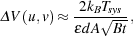 |
(24) |
where є is the efficiency of the system, dA is the station area, B is the bandwidth and t is the observation time (see e.g., [133]). This expression is simple to understand in that the more one observes – either in terms of integration time, frequency bandwidth or station collecting area – the less uncertainty one has. Obviously, if the signal we are after is well localized in either time, space or frequency the relevant noise calculation should take that into account.
In order to calculate the noise in the 3D power spectrum, the main
quantity we are after, one should remember that the frequency
direction in the observed datacube can be mapped one-to-one with the
redshift,
which in turn can be easily translated to distance, whereas the u and v
coordinates are in effect Fourier space coordinates. Therefore, to
calculate the power spectrum one should first Fourier transform the
data cube along the frequency direction. Following Morales' work
[133]
I will call the new Fourier space coordinate
 (with
d
resolution), which together with u and v defines the Fourier space
vector u = {u, v,
}. From
this, one can calculate the noise contribution to the power spectrum at
a given |u|,
(with
d
resolution), which together with u and v defines the Fourier space
vector u = {u, v,
}. From
this, one can calculate the noise contribution to the power spectrum at
a given |u|,
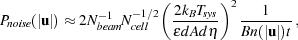 |
(25) |
where Nbeam is the number of simultaneous beams that could be measured, Ncell is the number of independent Fourier samplings per annulus and n(|u|) is the number of baselines covering this annulus [133]. Note that n(|u|) is proportional to the square of the number of stations, hence, n(|u|) dA2 is proportional to the square of the total collecting area of the array regardless of the station size. This means that in rough terms the noise power spectrum measurement does not depend only on the total collecting area, bandwidth and integration time, it also depends the number of stations per annulus. This is easy to understand as follows. The power in a certain Fourier space annulus is given by the variance of the measured visibilities in the annulus which carries uncertainty proportional to the inverse square root of the number of points. This point is demonstrated in Figure 20 [133, 134, 228].
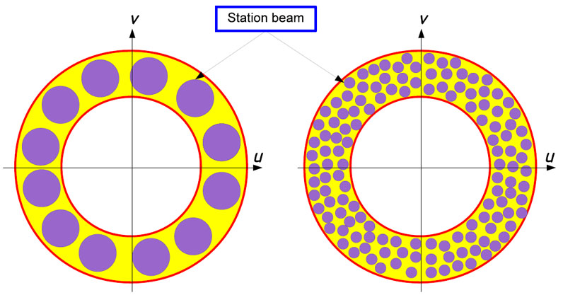 |
Figure 20. This figure shows how two different experiments might sample an annulus in the uv plane. The size of uv point is given by the station (interferometric element) size where a larger station (left hand panel) has a larger footprint relative to the smaller station case (right hand panel) in the uv plane; the footprint is shown by the purple circles. Even though the sampled area in the two cases might be the same, the fact that smaller stations sample the annulus more results in an increased accuracy in their estimation of the power spectrum. |
The foregrounds in the frequency regime (40-200MHz) are very bright and dominate the sky. In fact the amplitude of the foreground contribution, Tsky, at 150 MHz is about 4 orders of magnitude larger than that of the expected signal. However, since we are considering radio interferometers the important part of the foregrounds is that of the fluctuations and not the mean signal, which reduces the ratio between them and the cosmological signal to about 2-3 orders of magnitude, which is still a formidable obstacle to surmount.
The most prominent foreground is the synchrotron emission from relativistic electrons in the Galaxy: this source of contamination contributes about 75% of the foregrounds. Other sources that contribute to the foregrounds are radio galaxies, galaxy clusters, resolved supernovae remnants and free-free emission, which together provide 25% of the foreground contribution (see e.g., [182]). Figure 21 shows the simulated foreground contribution at 120 MHz taking into account all the foreground sources mentioned.
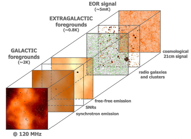 |
Figure 21. A figure showing the various cosmological and galactic components that contribute to the measured signal at a given frequency. The slices are color coded with different color tables owing to the vast difference in the range of brightness temperature in each component. The figure also shows the rms of the galactic foregrounds, extra galactic foregrounds and cosmological signal. |
Observationally, the regime of frequencies relevant to the EoR is obviously not very well explored. There are several all-sky maps of the total Galactic diffuse radio emission at different frequencies and angular resolutions. The 150 MHz map of Landecker & Wielebinski [104] is the only all-sky map in the frequency range (100-200 MHz) relevant for the EoR experiments, but has only 5° resolution.
In addition to current all-sky maps, a number of recent dedicated observations have given estimates of Galactic foregrounds in small selected areas.For example, Ali et al. [5] have used 153 MHz observations with GMRT to characterize the visibility correlation function of the foregrounds. Rogers and Bowman ([171]) have measured the spectral index of the diffuse radio background between 100 and 200 MHz. Pen et al. ([158]) have set an upper limit to the diffuse polarized Galactic emission.
Recently, a comprehensive program was initiated by the LOFAR-EoR collaboration to directly measure the properties of the Galactic radio emission in the frequency range relevant for the EoR experiments. The observations were carried out using the Low Frequency Front Ends (LFFE) on the WSRT radio telescope. Three different fields were observed. The first field was a highly polarized region known as the Fan region in the 2nd Galactic quadrant at a low Galactic latitude of ~ 10° [13]. This field is not ideal for measuring the EoR but it is a good field to learn from about calibration issues and about the influence of strong polarization.
The second field was a very cold region in the Galactic halo (l ~ 170°) around the bright radio quasar 3C196, and the third was a region around the North Celestial Pole (NCP) [14]. In the Fan region fluctuations of the Galactic diffuse emission were detected at 150 MHz for the first time (see Fig. 22). The fluctuations were detected both in total and polarized intensity, with an rms of 14 K (13 arcmin resolution) and 7.2 K (4 arcmin resolution) respectively [13]. Their spatial structure appeared to have a power law behavior with a slope of -2.2 ± 0.3 in total intensity and -1.65 ± 0.15 in polarized intensity (see Fig. 22). Note that, due to its strong polarized emission, the "Fan region" is not a representative part of the high Galactic latitude sky.
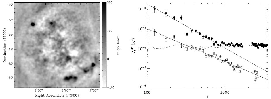 |
Figure 22. Left hand panel: Stokes I map of
the Galactic emission in the so-called Fan region, at Galactic
coordinates l = 137° and b = +8° in
the 2nd Galactic quadrant
[32,
80].
The conversion factor is
from flux (Jansky) to temperature is 1 Jy beam-1 = 105.6
K. Right hand panel: power spectrum (filled circles: total intensity;
asterisks: polarized intensity) of the Galactic emission in Fan region
with the best power-law fit. The plotted 1
|
The foregrounds in the context of the EoR measurements have been studied theoretically by various authors [182, 51, 50, 47, 176, 95, 71, 213, 49, 192, 210, 191, 26]. The first comprehensive simulation of the EoR foregrounds was carried out by Jelic et al. ([95]) focusing on the LOFAR-EoR project. The Jelic et al. model takes into account the Galactic diffuse synchrotron & free-free emission, synchrotron emission from Galactic supernova remnants and extragalactic emission from radio galaxies and clusters, both in total intensity and polarization. The simulated foreground maps, in their angular and frequency characteristics, are similar to the maps expected from the LOFAR-EoR experiment (see Fig. 21).
One major problem faced when considering the LOFAR-EoR data is disentangling the desired cosmological signal from the foreground signals. Even though the foregrounds are very prominent they are very smooth along the frequency direction [182, 95, 94, 13, 14], as opposed to the cosmological signal that fluctuates along the same direction. Hence, the separation of the two is, at a first glance, very simple. One would fit a smooth function to the data along the frequency direction and subtract it to obtain the desired signal. In reality, however, things are much more complicated as the existence of thermal noise and systematic errors due to calibration imperfections make the extraction much harder. In addition, the foregrounds are partially polarized, with a complicated structure along the frequency direction. The confluence of this with the ionospheric distortions and the polarized instrumental response makes it imperative to calibrate the data very accurately over a very wide field in order to obtain a very high dynamic range of observations. These factors make the fitting non-trivial, that might result in either under-fitting or over-fitting the signal. In the former case the deduced signal retains a large contribution of the foregrounds and produce a spurious "signal". Whereas in the over-fitting case one fits out the foregrounds and some of the signal resulting in an underestimation of the cosmological signal.
The simplest method for foreground removal in total intensity as a function of frequency is a polynomial fitting performed on the log-log scale which reduces to a power law in the first order case [95]. However, one should be careful in choosing the order of the polynomial to perform the fitting. If the order of the polynomial is too small, the foregrounds will be under-fitted and the EoR signal could be dominated and corrupted by the fitting residuals, while if the order of the polynomial is too big, the EoR signal could be fitted out. Arguably, it would be better to fit the foregrounds non-parametrically, i.e., allowing the data to determine their shape rather than selecting some functional form in advance and then fitting its parameters (see [79]).
After foreground subtraction from the EoR observations,
the residuals will be dominated by instrumental
noise, i.e., the level of the noise is expected to be an order of magnitude
larger than the EoR signal (assuming 300 hours of observation with
LOFAR). Thus, general statistical properties of the noise should be
determined and used to statistically detect the cosmological 21 cm
signal, e.g., the variance of the EoR signal over the image,
 EoR2,
as a function of frequency (redshift) obtained by
subtracting the variance of the noise,
noise2,
from that of the residuals,
residuals2. It has been
shown the such statistical detection of the EoR signal using the
fiducial model of the LOFAR-EoR experiment is possible
[95]
(see Figure 23).
Similar results by using different statistics are
the skewness of the one-point distribution of brightness temperature of the
EoR signal, measured as a function of observed frequency
[78],
and the power spectrum of variations in the intensity of redshifted 21 cm
radiation from the EoR
[77].
EoR2,
as a function of frequency (redshift) obtained by
subtracting the variance of the noise,
noise2,
from that of the residuals,
residuals2. It has been
shown the such statistical detection of the EoR signal using the
fiducial model of the LOFAR-EoR experiment is possible
[95]
(see Figure 23).
Similar results by using different statistics are
the skewness of the one-point distribution of brightness temperature of the
EoR signal, measured as a function of observed frequency
[78],
and the power spectrum of variations in the intensity of redshifted 21 cm
radiation from the EoR
[77].
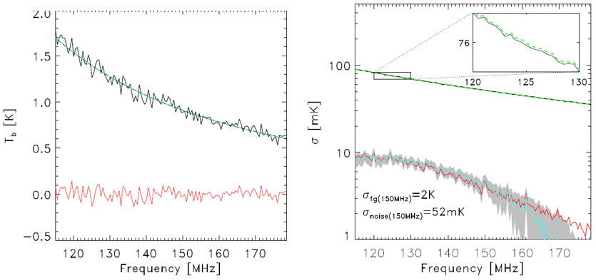 |
Figure 23. This figure shows the ability to
statistically extract the EoR signal from the foregrounds. Please
notice the difference in the vertical axis units between the two panels.
Left hand panel: One line of sight (one pixel along frequency) of the
LOFAR-EoR data maps (black solid line), smooth component of the
foregrounds (dashed black line), fitted foregrounds (dashed cyan line)
and residuals (red solid line) after taking out of the foregrounds.
Right hand panel: Statistical detection of the EoR signal
from the LOFAR-EoR data maps that include diffuse components of the
foregrounds and realistic instrumental noise
( |
2 Giant Metrewave Telescope, http://gmrt.ncra.tifr.res.in Back.
3 Low Frequency Array, http://www.lofar.org Back.
4 Murchinson Widefield Array, http://www.mwatelescope.org/ Back.
5 21 Centimeter Array, http://21cma.bao.ac.cn/ Back.
6 Precision Array to Probe EoR, http://astro.berkeley.edu/~dbacker/eor Back.
7 Square Kilometer Array, http://www.skatelescope.org/ Back.