Copyright © 2012 by Annual Reviews. All rights reserved
| Annu. Rev. Astron. Astrophys. 2012. 50:531-608
Copyright © 2012 by Annual Reviews. All rights reserved |


The interstellar medium (ISM) is a complex environment encompassing a very wide range of properties (e.g., McKee & Ostriker 1977; Cox 2005). In the Milky Way, about half the volume is filled by a hot ionized medium (HIM) with n < 0.01 cm-3 and TK > 105 K, and half is filled by some combination of warm ionized medium (WIM) and warm neutral medium (WNM), with n ~ 0.1 - 1 cm-3 and TK of several thousand K (Cox 2005). The neutral gas is subject to a thermal instability that predicts segregation into the warm neutral and cold neutral media (CNM), the latter with n > 10 cm-3 and TK < 100 K (Field et al. 1969). The existence of the CNM is clearly revealed by emission in the hyperfine transition of HI, with median temperature about 70 K, determined by comparison of emission to absorption spectra (Heiles & Troland 2003). However, the strict segregation into cold and warm stable phases is not supported by observations suggesting that about 48% of the WNM may lie in the thermally unstable phase (Heiles & Troland 2003). Finally, the molecular clouds represent the coldest (TK ~ 10 K in the absence of star formation), densest (n > 30 cm-3) part of the ISM. We focus on the cold (TK < 100 K) phases here, as they are the only plausible sites of star formation. The warmer phases provide the raw material for the cold phases, perhaps through "cold" flows from the intergalactic medium (Dekel & Birnboim 2006). In the language of this review, such flows would be "warm."
In the next section, we introduce some terminology used for the molecular gas as a precursor to the following discussion of the methods for tracing it. We then discuss the use of dust as a tracer (§ 2.3) before discussing the gas tracers themselves (§ 2.4).
2.2. Clouds and Their Structures
The CNM defined in the preceding section presents a wide array of structures, with a rich nomenclature, but we focus here on the objects referred to as clouds, invoking a kind of condensation process. This name is perhaps even more appropriate to the molecular gas, which corresponds to a change in chemical state.
The molecular cloud boundary is usually defined by the detection, above some threshold, of emission from the lower rotational transitions of CO. Alternatively, a certain level of extinction of background stars is often used. In confused regions, velocity coherence can be used to separate clouds at different distances along the line of sight. However, molecular clouds are surrounded by atomic envelopes and a transition region in which the hydrogen is primarily molecular, but the carbon is mostly atomic (van Dishoeck & Black 1988). These regions are known as PDRs, which stands either for Photo-Dissociation Regions, or Photon-Dominated Regions (Hollenbach & Tielens 1997). More recently, they have been referred to as "dark gas."
The structure of molecular clouds is complex, leading to considerable nomenclatural chaos. Cloud projected boundaries, defined by either dust or CO emission or extinction, can be characterized by a fractal dimension around 1.5 (Falgarone et al. 1991; Scalo 1990; Stutzki et al. 1998), suggesting an intrinsic 3-D dimension of 2.4. When mapped with sufficient sensitivity and dynamic range, clouds are highly structured, with filaments the dominant morphological theme; denser, rounder cores are often found within the filaments (e.g., André et al. 2010; Men'shchikov et al. 2010; Molinari et al. 2010).
The probability distribution function of surface densities, as mapped by extinction, can be fitted to a lognormal function for low extinctions, AV ≤ 2-5 mag (Lombardi et al. 2010), with a power law tail to higher extinctions, at least in some clouds. In fact, it is the clouds with the power-law tails that have active star formation (Kainulainen et al. 2009). Further studies indicate that the power-law tail begins at Σmol ~ 40-80 M⊙ pc-2, and that the material in the power-law tail lies in unbound clumps with mean density about 103 cm-3 (Kainulainen et al. 2011).
Within large clouds, and especially within the filaments, there may be small cores, which are much less massive but much denser. Theoretically, these are the sites of formation of individual stars, either single or binary (Williams et al. 2000). Their properties have been reviewed by di Francesco et al. (2007) and Ward-Thompson et al. (2007a). Those cores without evidence of ongoing star formation are called starless cores, and the subset of those that are gravitationally bound are called prestellar cores. Distinguishing these two requires a good mass estimate, independent of the virial theorem, and observations of lines that trace the kinematics. A sharp decrease in turbulence may provide an alternative way to distinguish a prestellar core from its surroundings (Pineda et al. 2010a).
While clouds and cores are reasonably well defined, intermediate structures are more problematic. Theoretically, one needs to name the entity that forms a cluster. Since large clouds can form multiple (or no) clusters, another name is needed. Williams et al. (2000) established the name "clump" for this structure. The premise was that this region should also be gravitationally bound, at least until the stars dissipate the remaining gas. Finding an observable correlative has been a problem (§ 2.5).
Finally, one must note that this hierarchy of structure is based on relatively large clouds. There are also many small clouds (Clemens & Barvainis 1988), some of which are their own clumps and/or cores. The suggestion by Bok & Reilly (1947) that these could be the sites of star formation was seminal.
In the Milky Way, roughly 1% of the ISM is found in solid form, primarily silicates and carbonaceous material (Draine 2003) (see also a very useful website 1). Dust grain sizes range from 0.35 nm to around 1 µm, with evidence for grain growth in molecular clouds. The column density of dust can be measured by studying either the reddening (using colors) or the extinction of starlight, using star counts referenced to an unobscured field. The relation between extinction (e.g., AV) and reddening [e.g., E(B - V)] is generally parameterized by RV = AV / E(B - V). In the diffuse medium, the reddening has been calibrated against atomic and molecular gas to obtain N(HI) + 2N(H2) = 5.8 × 1021 cm-2 E(B - V)(mag), not including helium (Bohlin et al. 1978). For RV = 3.1, this relation translates to N(HI) + 2N(H2) = 1.87 × 1021 cm-2 AV(mag). This relation depends on metallicity, with coefficients larger by factors of about 4 for the LMC and 9 for the SMC (Weingartner & Draine 2001).
The relation derived for diffuse gas is often applied in molecular clouds, but grain growth flattens the extinction curve, leading to larger values of RV, and a much flatter curve in the infrared (Flaherty et al. 2007; Chapman et al. 2009). More appropriate conversions can be found in the curves for RV = 5.5 in the website referenced above. There is evidence of continued grain growth in denser regions, which particularly affects the opacity at longer wavelengths, such as the mm/submm regions (Shirley et al. 2011).
Reddening and extinction of starlight provided early evidence of the existence of interstellar clouds (Barnard 1908). Lynds (1962) provided the mostly widely used catalog of "dark clouds" based on star counts, up to AV ~ 6 mag, at which point the clouds were effectively opaque at visible wavelengths. The availability of infrared photometry for large numbers of background stars from 2MASS, ISO, and Spitzer toward nearby clouds has allowed extinction measurements up to AV ~ 40 mag. These have proved very useful in characterizing cloud structure and in checking the gas tracers discussed in § 2.4. Extinction mapping with sufficiently high spatial resolution can identify cores (e.g., Alves et al. 2007), but many are not gravitationally bound (Lada et al. 2008), and they are likely to dissipate.
At wavelengths with strong, diffuse Galactic background emission, such as the mid-infrared, dust absorption against the continuum can be used in a way parallel to extinction maps (e.g., Bacmann et al. 2000; Stutz et al. 2007). The main uncertainties in deriving the gas column density are the dust opacity in the mid-infrared and the fraction of foreground emission.
The energy absorbed by dust at short wavelengths is emitted at longer wavelengths, from infrared to millimeter, with a spectrum determined by the grain temperature and the opacity as a function of wavelength. At wavelengths around 1 mm, the emission is almost always optically thin and close to the Rayleigh-Jeans limit for modest temperatures. (For Td = 20K, masses, densities, etc. derived in the Rayleigh-Jeans limit at λ = 1 mm must be multiplied by 1.5). Thus, the millimeter-wave continuum emission provides a good tracer of dust (and gas, with knowledge of the dust opacity) column density and mass.
As a by-product of studies of the CMB, COBE, WMAP, and Planck produce large-scale maps of mm/submm emission from the Milky Way. With Planck, the angular resolution reaches θ = 4.7 at 1.4 mm in an all-sky map of dust temperature and optical depth (Planck Collaboration et al. 2011b). Mean dust temperature increases from Td = 14 -15 K in the outer Galaxy to 19 K around the Galactic center. A catalog of cold clumps with Td = 7 - 17 K, mostly within 2 kpc of the Sun, many with surprisingly low column densities, also resulted from analysis of Planck data (Planck Collaboration et al. 2011c). Herschel surveys will be providing higher resolution [25" at 350 µm (Griffin et al. 2010) and 6" at 70 µm (Poglitsch et al. 2010)] images of the nearby clouds (André et al. 2010), the Galactic Plane (Molinari et al. 2010), and many other galaxies (e.g., Skibba et al. 2011; Wuyts et al. 2011). Still higher resolution is available at λ ≥ 350 µm from ground-based telescopes at dry sites. Galactic plane surveys at wavelengths near 1 mm have been carried out in both hemispheres (Aguirre et al. 2011; Schuller et al. 2009). Once these are put on a common footing, we should have maps of the Galactic plane with resolution of 20" to 30". Deeper surveys of nearby clouds (Ward-Thompson et al. 2007b), the Galactic Plane, and extragalactic fields are planned with SCUBA-2.
While studies from ground-based telescopes offer higher resolution, the need to remove atmospheric fluctuations leads to loss of sensitivity to structures larger than typically about half the array footprint on the sky (Aguirre et al. 2011). While the large-scale emission is lost, the combination of sensitivity to a minimum column density and a maximum size makes these surveys effectively select structures of a certain mean volume density. In nearby clouds, these correspond to dense cores (Enoch et al. 2009). For Galactic plane surveys, sources mainly correspond to clumps but can be whole clouds at the largest distances (Dunham et al. 2011b).
One troublesome aspect of extragalactic studies has been the determination of the amount and properties of the gas. We discuss first the atomic phase, then the molecular phase, and finally tracers of dense gas.
The cold, neutral atomic phase is traced by the hyperfine transition of hydrogen, occuring at 21 cm in the rest frame. This transition reaches optical depth of unity at
 |
(4) |
where Tspin is the excitation temperature, usually equal to the kinetic temperature, TK, and σv is the velocity dispersion (eq. 8.11 in Draine 2011). For dust in the diffuse ISM of the Milky Way, this column density corresponds to AV = 0.24 mag, and optical depth effects can be quite important. The warm, neutral phase is difficult to study, as lines become broad and weak, but it has been detected (Kulkarni & Heiles 1988). A detailed analysis of both CNM and WNM can be found in Heiles & Troland (2003).
With I(HI) = ∫Sνdv (Jy km s-1),
 |
(5) |
not including helium (eq. 8.21 in Draine 2011, but note errata regarding (1 + z) factor, which was in the numerator in the 2011 edition). A coefficient of 2.356 × 10⁵ is in common use among HI observers (e.g., Walter et al. 2008; Catinella et al. 2010; Giovanelli et al. 2005; Meyer et al. 2004), usually traced to Roberts (1975). The difference is almost certainly caused by a newer value for the Einstein A value in Draine (2011).
The most abundant molecule is H2, but its spectrum is not a good tracer of the mass in molecular clouds. The primary reason is not, as often stated, the fact that it lacks a dipole moment, but instead the low mass of the molecule. The effect of low mass is that the rotational transitions require quite high temperatures to excite, making the bulk of the H2 in typical clouds invisible. Continuum optical depth at the mid-infrared wavelengths of these lines is also an impediment. The observed rotational H2 lines originate in surfaces of clouds, probing 1% to 30% of the gas in a survey of galaxies (e.g., Roussel et al. 2007).
Carbon monoxide (CO) is the most commonly used tracer of molecular gas because its lines are the strongest and therefore easiest to observe. These advantages are accompanied by various drawbacks, which MW observations may help to illuminate. Essentially, CO emission traces column density of molecular gas only over a very limited dynamic range. At the low end, CO requires protection from photodissociation and some minimum density to excite it, so it does not trace all the molecular (in the sense that hydrogen is in H2) gas, especially if metallicity is low. At the high end, emission from CO saturates at modest column densities. A more complete review by A. Bolatto of the use of CO to trace molecular gas is scheduled for a future ARAA, so we briefly highlight the issues here.
CO becomes optically thick at very low total column densities. Using CO intensity to estimate the column density of a cloud is akin to using the presence of a brick wall to estimate the depth of the building behind it. The isotopologues of CO (13CO and C18O) provide lower optical depths, but at the cost of weaker lines. To use these, one needs to know the isotope ratios; these are fairly well known in the Milky Way (Wilson & Rood 1994), but they may differ substantially in other galaxies. In addition, the commonly observed lower transitions of CO are very easily thermalized (Tex = TK) making them insensitive to the presence of dense gas.
The common practice in studies of MW clouds is to use a combination of CO and 13CO to estimate optical depth and hence CO column density (N(CO)). One can then correlate N(CO) or its isotopes against extinction to determine a conversion factor (Dickman 1978; Frerking et al. 1982). A recent, careful study of CO and 13CO toward the Taurus molecular cloud shows that N(CO) traces AV up to 10 mag in some regions but only up to 4 mag in other regions, and other issues cause problems below AV = 3 mag (Pineda et al. 2010b). Freeze-out of CO and conversion to CO2 ice causes further complications in cold regions of high column density (Lee et al. 2003; Pontoppidan et al. 2008; Whittet et al. 2007), but other issues likely dominate the interpretational uncertainties for most extragalactic CO observations.
Since studies of other galaxies generally have only CO observations available, the common practice has been to relate H2 column density (N(H2)) to the integrated intensity of CO [I(CO) = ∫T dv (K km s-1)] via the infamous "X-factor": N(H2) = X(CO) I(CO). For example, Kennicutt (1998b) used X(CO) = 2.8 × 1020 cm-2 (K km s-1)-1.
Pineda et al. (2010b) find X(CO) = 2.0 × 1020 cm-2 (K km s-1)-1 in the parts of the cloud where both CO and 13CO are detected along individual sight lines. CO does emit beyond the area where 13CO is detectable and even, at a low level, beyond the usual detection threshold for CO. Stacking analysis of positions beyond the usual boundary of the Taurus cloud suggest a factor of two additional mass in this transition region (Goldsmith et al. 2008). Such low intensity, but large area, emission could contribute substantially to observations of distant regions in our galaxy and in other galaxies. For the outer parts of clouds, where only CO is detected, and only by stacking analysis, X(CO) is six times higher (Pineda et al. 2010b). Even though about a quarter of the total mass is in this outer region, they argue that the best single value to use is X(CO) = 2.3 × 1020 cm-2 (K km s-1)-1, similar to values commonly adopted in extragalactic studies. When possible, we will use X(CO) = 2.3 × 1020 cm-2 (K km s-1)-1 for this paper. In contrast, Liszt et al. (2010) argue that X(CO) stays the same even in diffuse gas. If they are right, much of the integrated CO emission from some parts of galaxies could arise in diffuse, unbound gas.
Comparing to extinction measures in two nearby clouds extending up to AV = 40 mag, Heiderman et al. (2010) found considerable variations from region to region, with I(CO) totally insensitive to increased extinction in many regions. Nonetheless, when averaged over the whole cloud, the standard X(CO) would cause errors in mass estimates of ± 50%, systematically overestimating the mass for Σmol < 150 M⊙ pc-2 and underestimating for Σmol > 200 M⊙ pc-2. Simulations of turbulent gas with molecule formation also suggest that I(CO) can be a very poor tracer of AV (Glover et al. 2010). Overall, the picture at this point is that measuring the extent of the brick wall will not tell you anything about particularly deep or dense extensions of the building, but if the buildings are similar, the extent of the wall is a rough guide to the total mass of the building (cf. Shetty et al. 2011b).
Following that thought, the luminosity of CO J = 1 → 0 is often used as a measure of cloud mass, with the linewidth reflecting the virial theorem in a crude sense. In most extragalactic studies, individual clouds are not resolved, and the luminosity of CO is essentially a cloud counting technique (Dickman et al. 1986). Again, this idea works only if the objects being counted have rather uniform properties. In this approach, M = αCO L(CO). For the standard value for X(CO) discussed above (X(CO) = 2.3 × 1020 cm-2 (K km s-1)-1) αCO = 3.6 M⊙(K km s-1 pc2)-1 without helium, and αCO = 4.6 M⊙(K km s-1 pc2)-1 with correction for helium.
The effects of cloud temperature, density, metallicity, etc. on mass estimation from CO were discussed by Maloney & Black (1988), who concluded that large variations in the conversion factor are likely. Ignoring metallicity effects, they would predict X(CO) ∝ n0.5 TK-1, where n is the mean density in the cloud. Shetty et al. (2011b) find a weaker dependence on TK, X(CO) ∝ TK-0.5. These scalings rests on some arguments that may not apply in other galaxies. Further modeling with different metallicities (Shetty et al. 2011a; Feldmann et al. 2012) has begun to provide some perspective on the range of behaviors likely in other galaxies.
There is observational evidence for changes in αCO in centers of galaxies. In the MW central region, Oka et al. (1998) suggest a value for X(CO) a factor of 10 lower than in the MW disk. The value of αCO appears to decrease by factors of 2-5 in nearby galaxy nuclei (e.g., Meier & Turner 2004; Meier et al. 2008), and by a factor of about 5-6 in local ULIRGs (Downes & Solomon 1998; Downes et al. 1993), and probably by a similar factor in high-redshift, molecule-rich galaxies (Solomon & Vanden Bout 2005).
A compilation of measurements indicates that αCO decreases from the usually assumed value with increasing surface density of gas once Σmol > 100 M⊙ pc-2 (Fig. 1, Tacconi et al. 2008). This Σmol corresponds to AV ~ 10 mag, about the point where CO fails to trace column density in Galactic clouds, and the point where the beam on another galaxy might be filled with CO-emitting gas. Variation in αCO has a direct bearing on interpretation of starbursts (§ 6), and it is highly unlikely that αCO is simply bimodal over the full range of star forming environments. Indeed, Narayanan et al. (2012) use a grid of model galaxies to infer a smooth function of I(CO): αCO = min[6.3, 10.7 × I(CO)-0.32] Z′ -0.65, where Z′ is the metallicity divided by the solar value.
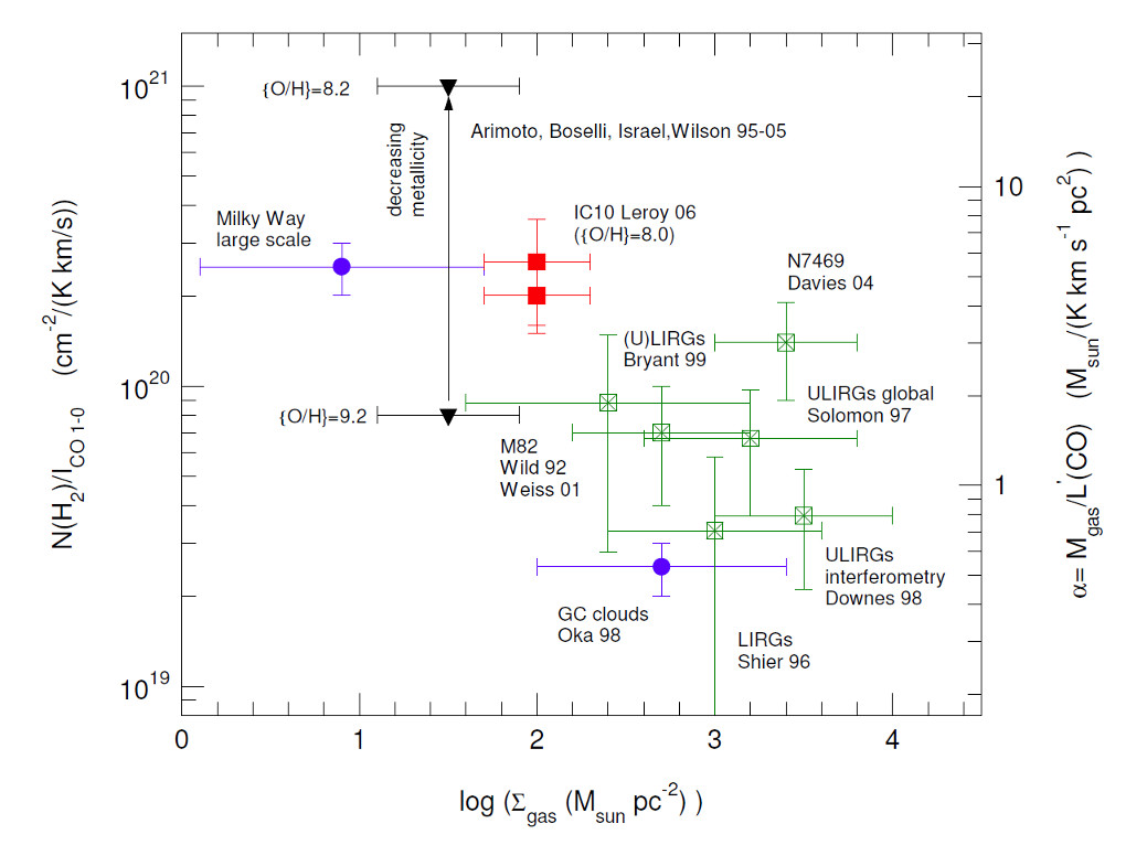 |
Figure 1. Compilation of the conversion factor (X(CO)) from the CO J = 1 → 0 integrated intensity [ICO (K km s-1)] or luminosity [L'CO (K km s-1 pc2)] to H2 column density (left vertical scale) and total (H2 and He) gas mass (right vertical scale), derived in various Galactic and extragalactic targets. Blue circles denote measurements in the disk and center of the MilkyWay, based on various virial, extinction, and isotopomeric analyses. Crossed green squares denote measurements in starbursts and (U)LIRGs, mainly based on dynamical constraints. Filled triangles denote conversion factors as a function of decreasing metallicity (vertical arrow) from (bottom) to 8.2 (top), derived mainly from global (large scale) dust mass measurements in nearby galaxies and dwarfs by several groups. In contrast, red filled squares mark X-factor measurements toward individual clouds, over the same range in metallicity. Taken from Tacconi et al. (2008); references to the original work are given there. Reproduced by permission of the AAS. |
Other methods have been used to trace gas indirectly, including gamma-ray emission and dust emission. Gamma-rays from decay of pions produced from high-energy cosmic rays interacting with baryons in the ISM directly trace all the matter if one knows the cosmic ray flux (e.g., Bloemen 1989). Recent analysis of gamma-ray data from Fermi have inferred a low value for X(CO) of (0.87 ± 0.05) × 1020 cm-2 (K km s-1)-1 in the solar neighborhood (Abdo et al. 2010). This value is a factor of three lower than other estimates and early results from dust emission, using Planck, which found X(CO) = (2.54 ± 0.13) × 1020 cm-2 (K km s-1)-1 for the solar neighborhood. (Planck Collaboration et al. 2011b).
Abdo et al. (2010) also inferred the existence of "dark gas", which is not traced by either HI or CO, surrounding the CO-emitting region in the nearby Gould Belt clouds, with mass of about half of that traced by CO. Planck Collaboration et al. (2011b) have also indicated the existence of "dark gas" with mass 28% of the atomic gas and 118% of the CO-emitting gas in the solar neighborhood. The dark gas appears around AV = 0.4 mag, and is presumably the CO-poor, but H2-containing, outer parts of clouds (e.g., Wolfire et al. 2010), which can be seen in [CII] emission at 158 and in fluorescent H2 emission at 2 (e.g., Pak et al. 1998). It is dark only if one restricts attention to HI and CO. At low metallicities, the layer of C+ grows, and a given CO luminosity implies a larger overall cloud (see Fig. 14 in Pak et al. 1998). However, Planck Collaboration et al. (2011b) also suggest that the dark gas may include some gas that is primarily atomic, but not traced by HI emission, owing to optical depth effects.
Dust emission is now being used as a tracer of gas for other galaxies. Maps of HI gas are used to break the degeneracy between the gas to dust ratio δgdr and α′CO in the following equation:
 |
(6) |
Leroy et al. (2011) minimize the variation in δgdr to find the best fit to α′CO in several nearby galaxies. They determine Σdust from Spitzer images of 160 emission, with the dust temperature (or equivalently the external radiation field) constrained by shorter wavelength far-infrared emission. This method should measure everything with substantial dust that is not HI, so includes the so-called "dark molecular gas." They find that α′CO = 3 - 9 M⊙ pc-2 (K km s-1)-1, similar to values based on MW studies, for galaxies with metallicities down to 12 + [O/H] ~ 8.4, below which α′CO increases sharply to values like 70. Their method does not address the column density within clouds, but only the average surface density on scales larger than clouds. For galaxies not too different from the MW, the standard α′CO will roughly give molecular gas masses, but in galaxies with lower metallicity, the effects can be large. An extreme is the SMC, where α′CO ~ 220 M⊙ pc-2 (K km s-1)-1 (Bolatto et al. 2011). Maps of dust emission at longer wavelengths should decrease the sensitivity to dust temperature.
Lines other than CO J = 1 → 0 generally trace warmer (e.g., higher J CO lines) and/or denser (e.g., HCN, CS, ...) gas. Wu et al. (2010a) showed that the line luminosities of commonly used tracers (CS J = 2 → 1, J = 5 → 4, and J = 7 → 6; HCN J = 1 → 0, J = 3 → 2) correlate well with the virial mass of dense gas; indeed most follow relations that are close to linear. Since these lines are optically thick, the linear correlation is somewhat surprising, but it presumably has an explanation similar to the cloud-counting argument offered above for CO. Collectively, we refer to these lines as "dense gas tracers", but the effective densities increase with J and vary among species (see Evans 1999; Reiter et al. 2011b for definitions and tables of effective and critical densities). As an example for HCN J = 1 → 0,
 |
(7) |
from a robust estimation fit to data on dense clumps in the MW (Wu et al. 2010a). The line luminosities of other dense gas tracers also show strong correlations with both virial mass (Wu et al. 2010a) and the mass derived from dust continuum observations (Reiter et al. 2011b).
These tracers of dense gas are of course subject to the same caveats about sensitivity to physical conditions, such as metallicity, volume density, turbulence, etc., as discussed above for CO. In fact, the other molecules are more sensitive to photodissociation than is CO, so they will be even more dependent on metallicity (e.g., Rosolowsky et al. 2011). Dense gas tracers should become much more widely used in the ALMA era, but caution is needed to avoid the kind of over-simplification that has tarnished the reputation of CO. Observations of multiple transitions and rare isotopes, along with realistic models, will help (e.g., García-Burillo et al. 2012).
What do extragalactic observations of molecular tracers actually measure? None are actually tracing the surface density of a smooth medium, with the possible exception of the most extreme starbursts. The luminosity of CO is a measure of the number of emitting structures times the mean luminosity per structure. Dense gas tracers work in a similar way, but select gas above a higher density threshold than does CO. For CO J = 1 → 0, the structure is the CO emitting part of a cloud, which shrinks as metallicity decreases. For dense gas tracers, the structure is the part of a cloud dense enough to produce significant emission, something like a clump if conditions are like the MW, but even more sensitive to metallicity. Using a conversion factor, one gets a "mass" in those structures.
Estimates of the conversion factors for CO vary by factors of 3 for the solar neighborhood and at least an order of magnitude at low metallicity and by at least half an order of magnitude for our own Galactic Center and for extreme systems like ULIRGs. Dividing by the area of the galaxy or the beam, one gets "Σmol", which really should be thought of as an area filling factor of the structures being probed times some crude estimate of the mass per structure. That estimate depends on conditions in the structures, such as density, temperature, and abundance and on the external radiation field and the metallicity. Once the L(CO) translates to surface densities above that of individual clouds (Σmol > ~ 100 M⊙ pc-2), the interpretation may change as the area filling factor can now exceed unity. Large ranges of velocity in other galaxies (if not exactly face-on) allow I(CO) to still count clouds above this threshold, but the clouds may no longer be identical. The full range of inferred molecular surface densities in other galaxies inferred from CO, assuming a constant conversion factor, is a factor of 103 (§ 6); given that CO traces Σmol only over a factor of 10 at best in well-studied clouds in the MW (Pineda et al. 2010b; Heiderman et al. 2010), this seems a dangerous extrapolation.
2.5. Mass Functions of Stars, Clusters, and Gas Structures
The mass functions of the structures in molecular clouds (§ 2.2) are of considerable interest in relation to the origin of the mass functions of clusters (clumps) and stars (cores). Salpeter (1955) fit the initial mass function (IMF) of stars to a power law in logM* with exponent γ* = 1.35, or α* = 2.35 (see § 1.2 for definitions). More recent determinations over a wider range of masses, including brown dwarfs, indicate a clear flattening at lower masses, either as broken power laws (Kroupa et al. 1993) or a log-normal distribution (Miller & Scalo 1979; Chabrier 2003). A detailed study of the IMF in the nearest massive young cluster, Orion, with stars from 0.1 to 50 M⊙ with a mean age of 2 Myr, shows a peak between 0.1 and 0.3 M⊙, depending on evolutionary models, and a deficit of brown dwarfs relative to the field IMF (Da Rio et al. 2012). Steeper IMFs in massive elliptical galaxies have been suggested by van Dokkum & Conroy (2011). Zinnecker & Yorke (2007) summarize the evidence for a real (not statistical) cut-off in the IMF around 150 M⊙ for star formation in the MW and Magellanic Clouds. Variations in the IMF with environment are plausible, but convincing evidence for variation remains elusive (Bastian et al. 2010).
The masses of embedded young clusters (Lada & Lada 2003), OB associations (McKee & Williams 1997), and massive open clusters (Elmegreen & Efremov 1997; Zhang & Fall 1999), follow a similar relation with γcluster ~ 1. Studies of clusters in nearby galaxies have also found γcluster = 1 ± 0.1, with a possible upper mass cutoff or turn-over around 1-2 × 10⁶ M⊙ (Gieles et al. 2006), perhaps dependent on the galaxy (but see Chandar et al. 2011). In contrast, the most massive known open clusters in the MW appear to have a mass of (6-8) × 104 M⊙ (Portegies Zwart et al. 2010; Davies et al. 2011; Homeier & Alves 2005).
The mass functions of clusters and stars are presumably related to the mass functions of their progenitors, clouds or clumps, and cores. For comparison to structures in clouds, we will use the distributions versus mass, rather than logarithmic mass, so our points of comparison will be α* = 2.3 and αcluster = 2. From surveys of emission from CO J = 1 → 0 in the outer galaxy, where confusion is less problematic, Heyer et al. (2001) found a size distribution of clouds, dN / dr ∝ r-3.2±0.1, with no sign of a break from the power-law form from 3 to 60 pc. The mass function, using the definition in equation 2, was fitted by αcloud = 1.8 ± 0.03 over the range 700 to 1 × 10⁶ M⊙. Complementary surveys of the inner Galaxy found αcloud = 1.5 up to Mmax = 106.5 M⊙ (Rosolowsky 2005). The upper cut-off around 3-6 × 10⁶ M⊙ appears to be real, despite issues of blending of clouds (Williams & McKee 1997; Rosolowsky 2005). Using 13CO J = 1 → 0, which selects somewhat denser parts of clouds, Roman-Duval et al. (2010) found α13CO = 1.75± 0.23 for Mcloud > 105 M⊙. Clumps within clouds, identified by mapping 13CO or C18O, have a similar value for αclump = 1.4-1.8 (Kramer et al. 1998). All results agree that most clouds are small, but, unlike stars or clusters, most mass is in the largest clouds (αcloud < 2).
Studies of molecular cloud properties in other galaxies have been recently reviewed (Fukui & Kawamura 2010; Blitz et al. 2007). Mass functions of clouds in nearby galaxies appear to show some differences, though systematic effects introduce substantial uncertainty (Wong et al. 2011; Sheth et al. 2008). Evidence for a higher value of αcloud has been found for the LMC (Fukui et al. 2001; Wong et al. 2011) and M33 (Engargiola et al. 2003; Rosolowsky (2005)). Most intriguingly, the mass function appears to be steeper in the interarm regions of M51 than in the spiral arms (E. Schinnerer and A. Hughes, personal communication), possibly caused by the aggregation of clouds into larger structures within arms and disaggregation as they leave the arms (Koda et al. 2009).
Much work has been done recently on the mass function of cores, and Herschel surveys of nearby clouds will illuminate this topic (e.g., André et al. 2010). At this point, it seems that the mass function of cores is clearly steeper than that of clouds, much closer to that of stars (Motte et al. 1998; Enoch et al. 2008; Sadavoy et al. 2010). A turnover in the mass function appears at a mass about 3-4 times that seen in the stellar IMF (Alves et al. 2007; Enoch et al. 2008). The similarity of αcore to α* supports the idea that the cores are the immediate precursors of stars and that the mass function of stars is set by the mass function of cores. In this picture, the offset of the turnover implies that about 0.2 to 0.3 of the core mass winds up in the star, consistent with simulations that include envelope clearing by outflows (e.g., Dunham et al. 2010). Various objections and caveats to this appealing picture have been registered (e.g., Swift & Williams 2008; Reid et al. 2010; Clark et al. 2007; Hatchell & Fuller 2008).
Note that no such tempting similarity exists between the mass function of clusters and the mass function of clumps defined by 13CO maps, questioning whether that observational definition properly fits the theoretical concept of a clump as a cluster-forming entity. Structures marked by stronger emission in 13CO or C18O (Rathborne et al. 2009) are not always clearly bound gravitationally. Ground and space-based imaging of submillimeter emission by dust (e.g., Men'shchikov et al. 2010) offer promise in this area, but information on velocity structure will also be needed. The data so far suggest that the structure is primarily filamentary, more like that of clouds than that of cores. CS, HCN and other tracers of much denser gas (§ 2.4), along with dust continuum emission (§ 2.3) have identified what might be called "dense clumps", which do appear to have a mass function similar to that of clusters (Shirley et al. 2003; Beltrán et al. 2006; Reid & Wilson 2005),
The comparison of mass functions supports the idea (McKee & Ostriker 2007) that cores are the progenitors of stars and dense clumps are the progenitors of clusters, with clouds less directly related. Upper limits to the mass function of clumps would then predict upper limits to the mass function of clusters, unless nearby clumps result in merging of clusters. Because most clouds and many clumps are more massive than the most massive stars, it is less obvious that an upper limit to stellar masses results from a limit on cloud or clump masses. If clump masses are limited and if the mass of the most massive star to form depends causally (not just statistically) on the mass of the clump or cloud, the integrated galactic IMF (IGIMF) can be steepened (Kroupa & Weidner 2003; Weidner & Kroupa 2006). We discuss the second requirement in § 4.2 and consequences of this controversial idea in § 3.3 and § 6.4.
1 http://www.astro.princeton.edu/~draine/dust/dust.html Back.