


In this section, we review measurements of the alignments of galaxies and groups/clusters of galaxies which have considered the specific environment in which such systems reside. At megaparsec scales, the cosmic web can be roughly divided into four different types of environments: voids, sheets, filaments, and knots. In numerical simulations, these environments are defined according to the number of gravitationally collapsed dimensions: 0, 1, 2, and 3, respectively. Voids correspond to the emptiest parts of the sky (in terms of galaxy density): underdense regions with scales of ≳10 Mpc; while knots correspond to massive galaxy groups and clusters (e.g., Hahn et al., 2007).
Alignment measurements that take into account the different environments started in the late 1960s with photographic plates and only in the 21st century did measurements start to be performed with modern CCD cameras. In the following sections we discuss the most recent results; a full historical review is presented in Joachimi et al. 2015.
In this section (particularly in Section 5.1 and 5.5) we take the distribution of satellite galaxies as an observational proxy for the shape of the host dark matter halo, which is not accessible to observations. This is a reasonable, although not exact, approximation for dark matter haloes with elliptical central galaxies, i.e. mostly groups and clusters (see Kiessling et al. 2015). It is probably not applicable to spiral (late-type) centrals; for such galaxies a coherent satellite distribution may hint to a common tidal origin of these satellites (e.g. Pawlowski & Kroupa, 2013).
For these observations it is of course important that galaxy type and the morphology of the local large-scale structure (groups, filaments, voids, sheets) are determined to high accuracy when attempting to make statements about galaxy shape correlation for a given population. Bailin et al., (2008) assessed different selection criteria for isolated and group galaxies using SDSS and the Millenium simulation (Springel et al., 2005) and showed that most studies correctly identified only ∼30−40% of isolated galaxies (and their satellites) in their samples, with the rest typically being incorrectly identified as members of galaxy groups. Improvements in identification are very important for the future of these studies. More discussion of the characterisation of morphology in N-body and hydrodynamical simulations can be found in Kiessling et al. (2015).
Some groups have made interesting attempts to use quasar polarisation as a tracer of alignment (Hutsemékers, 1998, Hutsemékers & Lamy, 2001, Hutsemékers et al., 2005). The unified picture of Active Galactic Nuclei (AGN), which include quasars, sees them as sourced by the accretion of matter onto a central supermassive black hole. The polarisation is believed to be either parallel or perpendicular to the accretion disc, depending on inclination with respect to the line of sight, based on studies of low redshift AGN (Smith et al., 2004). Hutsemékers et al., (2014) found that quasar polarization in galaxy groups at z ∼ 1.3 is either parallel or perpendicular to the principal axis defined by group galaxies, as well as being correlated with the polarisation vectors of their neighbouring quasars.
5.1. Galaxy position alignments in the field and the Local Group
Holmberg, (1969) originally found that the distribution of galaxies that are satellites around field spirals tend to be located along the minor axis of the central galaxy. He looked at edge-on spiral host galaxies, whose minor axes are easier to identify, and restricted himself to satellites at radii smaller than 50 kpc. Subsequent studies using larger samples of galaxies were not able to confirm this result (e.g. Hawley & Peebles, 1975, Sharp et al., 1979). Zaritsky et al., (1997) did find evidence for this “Holmberg effect”, but only for satellites at distances between 300 and 500 kpc from their host galaxy. Later studies using SDSS have found that satellites of spiral galaxies are distributed isotropically (e.g. Azzaro et al., 2007, Bailin et al., 2008). In contrast, satellites of early-type centrals are located preferentially along their host's major axes, i.e. an anti-Holmberg effect 2 (Brainerd, 2005, Azzaro et al., 2007, Sales & Lambas, 2009, Nierenberg et al., 2011).
Contrary to the results for field galaxies, there is evidence of a strong Holmberg effect for Milky Way satellites (e.g. Lynden-Bell, 1976, Kunkel & Demers, 1976, Kroupa et al., 2005, Pawlowski & Kroupa, 2013). M31 is probably the only galaxy other than the Milky Way for which the three-dimensional distribution of satellites can be mapped with accuracy because distances can be measured precisely. Koch & Grebel, (2006) found that early-type dwarf satellites of M31 are located in a polar plane, only 16 kpc thick, that is only ∼6∘ from the pole of M31. Similar findings have been presented by Conn et al., (2013) and Ibata et al. (2013). Pawlowski et al., (2013) have suggested that two similar structures can be found for non-satellite galaxies in the Local Group as a whole, at roughly equal distances to the Milky Way and M31.
As discussed by Bailin et al., (2008) these results need not be contradictory, for two reasons: firstly, the large spirals in the Local Group are not isolated as defined in the above SDSS studies, since M31 and the Milky Way are too close to one another to define either of them as “isolated”; secondly, the satellites of these galaxies are much fainter than the typical satellites of SDSS field galaxies. Indeed, Bailin et al., (2008) found a minor-axis alignment of sufficiently faint satellites around their hosts in hydrodynamical simulations.
5.2. Galaxy alignments within galaxy groups and clusters
Galaxy clusters can host hundreds of galaxies and have therefore attracted considerable attention since the pioneering works of Fritz Zwicky (e.g., Zwicky, 1933, Zwicky, 1937). SDSS data have been used to generate catalogues that contain hundreds of thousands of groups and clusters (e.g., Koester et al., 2007, Hao et al., 2010, Wen et al., 2012, Rykoff et al., 2014).
There is consistent evidence that the major axes of centrals in galaxy clusters, typically referred to as brightest cluster galaxies, BCGs, but different from these in some non-negligible fraction of cases (Skibba et al., 2015, Hoshino et al., 2015), seem to produce an inverted Holmberg effect; that is, the major axes of the central galaxy and the satellite distribution (which serves as an observational proxy for the shape of the cluster's dark matter halo) coincide to a good degree. This tendency has been evident since the very first measurements (Sastry, 1968, Rood & Sastry, 1972, Austin & Peach, 1974, Dressler, 1978, Carter & Metcalfe, 1980, Binggeli, 1982, Struble, 1987). The most recent measurements have come from analyses of large galaxy group/cluster catalogues from SDSS spectroscopic (Yang et al., 2006, Azzaro et al., 2007, Faltenbacher et al., 2007, Wang et al., 2008, Wang et al., 2010, Siverd et al., 2009) or photometric (Niederste-Ostholt et al., 2010, Hao et al., 2011) data, all of which have confirmed this alignment, which is typically found to be stronger for early-type, or red, central galaxies. The brightest satellite galaxies' shapes are also aligned with the parent halo (Li et al., 2013b, Singh et al., 2014), and there is evidence that BCGs are also aligned with the shape of the X-ray emission from the intracluster medium (Hashimoto et al., 2008). Using a sample of 405 Abell clusters, Struble, (1988) showed that pairs of brightest cluster galaxies tend to be aligned parallel to each other and perpendicular to the separation vector. This is at odds with more recents results which show alignment between clusters, discussed in Section 5.5 below.
On the other hand, as reviewed in Joachimi et al. 2015, historically there has not been a strong consensus about the alignments of satellite galaxy shapes within their host haloes (or the lack thereof). However, the latest measurements seem to agree that, on scales from small galaxy groups (M ∼ 1013 M⊙) to massive galaxy clusters (M ≳ 1015 M⊙), the orientations of satellite galaxies are consistent with an isotropic distribution (Sifón et al., 2015, Chisari et al., 2014) (probably with the exception of the brightest satellites, as described above).
The first modern (i.e., using CCD observations), statistical measurements of galaxy alignments in galaxy groups were presented by Pereira & Kuhn, (2005), who used SDSS photometric and spectroscopic observations and found anisotropic galaxy orientations at the 4σ level. Some other authors have also found that satellite galaxies are aligned either radially from the position of the central galaxy (Agustsson & Brainerd, 2006, Faltenbacher et al., 2007) or aligned with the major axis of the central galaxy (Yang et al., 2006). However, Hao et al. (2011) showed that these detections correspond to systematic effects in the isophotal measurements from SDSS. Since Hao et al. (2011), all measurements have been consistent with no alignments (Hung & Ebeling, 2012, Schneider et al., 2013, Chisari et al., 2014, Sifón et al., 2015). Chisari et al., (2014) presented a modelling of intrinsic alignments in photometrically selected groups and clusters, improving upon the method of Blazek et al., (2012) by accounting for photometric redshift errors using the full redshift probability distribution of each galaxy. In a complementary work, Sifón et al., (2015) used a large sample of spectroscopically-confirmed galaxy cluster members to directly measure the average alignment of satellite galaxies. The work of Chisari et al., (2014) has the advantage of being applicable to photometric data, with great potential for large photometric surveys such as the Large Synoptic Survey Telescope (LSST, LSST Science Collaboration et al., 2009) and Euclid (Laureijs et al., 2011), while that of Sifón et al., (2015) is a cleaner and more direct measurement but depends on large spectroscopic datasets which are less readily available. Both works found no evidence for galaxy alignments in clusters, constraining the average intrinsic ellipticity signal in galaxy groups and clusters to be 0.5% or lower. The measurements of Sifón et al., (2015) are reproduced in Figure 9; they used two different shape measurement methods with different radial weighting schemes (GALFIT, by Peng et al. 2002, and KSB, by Kaiser et al. 1995, see Section 2.3 above for more discussion of shape measurement methods), both of which gave consistent results, suggesting that the non-detection of alignments in clusters is robust to differences in shape measurement. Additionally, thanks to their large, clean sample of cluster members, Sifón et al., (2015) directly measured the alignment between cluster satellites, which they also found to be consistent with zero. The fact that the measurement of the cross component, ⟨ є× ⟩, was consistent with zero acts as a null test and demonstrates that the analysis of Sifón et al., (2015) is robust to, at least some types of, systematics. Also using spectroscopically-confirmed cluster members but with reduced constraining power due to lower image quality of single-pass SDSS observations (as opposed to deep SDSS Stripe 82 data and deep, better-seeing CFHT/MegaCam images used by Chisari et al. 2014 and Sifón et al. 2015, respectively), Schneider et al., (2013) constrained the average shear signal of satellite galaxies in Galaxy and Mass Assembly (GAMA) survey 3 (Driver et al., 2009) groups to ≲ 2%. Schneider et al., (2013) note the disagreement between their null detection and results from N-body simulations, suggesting that this is evidence for misalignment between baryonic and dark matter shapes.
 |
Figure 9. The average ellipticities, ⟨ єi⟩ (with i denoting the + or × ellipticity component), of galaxies in galaxy clusters from 14,250 spectroscopically-confirmed cluster members, using two different shape measurement methods on data from the CFHT, as a function of projected distance from the BCG, normalised to the cluster radius, r200 (note that r as used here is the same as rp used throughout this paper). KSB measure quadrupole moments of the brightness distribution (Kaiser et al., 1995), Galfit is a model-fitting method (Peng et al., 2002). Positive (negative) red circles represent radial (tangential) alignments, while the blue crosses show the cross component of the ellipticity. Dashed lines and shaded regions show the weighted mean and its 1, 2, and 3σ uncertainty regions for all galaxies within r200, and the white boxes show the results when including photometrically-selected red sequence members. Reproduced with permission from Sifón et al. (2015) © ESO. |
As discussed by Singh et al., (2014), the observed radial alignments of the most luminous satellite galaxies by Li et al., (2013b) and Singh et al., (2014) would lead to null detections of fainter satellites as observed by, for example, Chisari et al., (2014) and Sifón et al., (2015). This assumes that the scaling of satellite alignments with luminosity estimated by Singh et al., (2014) for bright red galaxies (specifically LRGs) is extrapolated below the luminosity limit explored by the latter authors, whose sample also incuded blue galaxies which would further dilute any signal. Therefore, to current precision, the latest observations show a consistent picture, in which very luminous (red) satellites align towards the central galaxy and progressively fainter (red and blue) satellites align less and less until the alignment signal of faint satellites is below the current detection limit.
5.3. Galaxy alignments with voids
Voids are an attractive reference against which alignments of galaxies can be measured. They have a higher degree of symmetry than filaments and, in contrast to clusters, tend to become more spherical as they evolve gravitationally – the effect of the strongest inward forces acting along the shortest axis in an aspherical overdensity is reversed for underdense voids (Sheth & van de Weygaert, 2004). On the downside, large voids are rare objects and are characterised by the absence of luminous structures, so detecting them requires a galaxy survey covering a large, contiguous volume with densely sampled spectroscopic redshifts.
Such a dataset only became available with the advent of SDSS, which additionally supplied imaging of sufficient quality to measure galaxy morphology with high accuracy. Thus it is not surprising that the observational study of void alignments closely follows the development of SDSS, with three publications based on DR3 (Trujillo et al., 2006), DR6 (Slosar & White, 2009), and DR7 (Varela et al., 2012). These works shared a lot of their methodology, in particular the algorithm to find and define voids (the HB algorithm described in Patiri et al. 2006 who also give an overview of other methods), but obtained strikingly different results. It is possible that details of the implementation, for example assumed limiting magnitudes, which differed between implementations of the same algorithm are responsible, underlining the sensitivity of void-finding to the method employed.
Trujillo et al. (2006) searched for alignments among galaxies on the surface of voids using data from SDSS DR3 and the Two-Degree Field Galaxy Redshift Survey (2dFGRS). They defined voids as spheres of radius larger than 10 Mpc/h (clearly an idealistic assumption, there will generally be some confusion over void boundaries) within the SDSS survey boundaries that contain no galaxies brighter than Mbj = −19.32 + 5 logh. Here, bj denotes a blue photometric band used for the target photometry of the 2dF Galaxy Redshift Survey (Colless et al., 2001). Disc-dominated galaxies were selected in a shell of 4 Mpc/h thickness on the surface of the voids, using only objects that are nearly face-on or edge-on. The latter step avoids an ambiguity in the inclination of the disc as it is impossible to decide which are the near and far edges of the galaxy if only the axis ratio of the image is known.
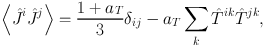
In total, Trujillo et al. (2006) used 178 voids and 201 galaxies with estimates of their spin axes. From these they derived the probability distribution of the angle θ between the spin vector of a galaxy and the vector connecting the void centre with the position of the galaxy. Their measurement is inconsistent with random galaxy orientations at the 99.7 % level, preferring an orientation of the spin vector perpendicular to the void radius vector. The signal is well described by a simple model based on tidal torque theory, assuming
 |
(30) |
where Ĵi is the normalised spin vector, Tij the normalised traceless shear tensor, i, j denote pairs of galaxies, and aT ∈ [0; 1.0] a correlation parameter measuring the alignment of the shear and inertia tensors (Lee & Pen, 2000). δij is the Kronecker delta. Based on this model for spin correlations, and assuming a Gaussian distribution of the spin vector elements, Lee (2004) derived a general result for the probability distribution of angles of galaxy spin vectors relative to eigenvectors of the tidal shear field which was able to qualitatively recover the observed inclinations of spiral galaxies in the local supercluster. Trujillo et al. (2006) measured aT = 0.7−0.2+0.1 (1σ).
This detection is in marked contrast to that of Slosar & White (2009) who reported a null detection with a constraint aT < 0.13 at 3σ. Their analysis only differed in that it was updated to the larger and more homogeneous DR6 and used an absolute magnitude limit 4 of Mr = −20.23 + 5 logh as the threshold for void detection. The larger area and higher filling factor for galaxies inside the survey volume resulted in a significantly larger sample of voids. Additionally, their definition of the galaxy sample on which spin measurements were made was slightly different, but even when approximately recovering the selection of Trujillo et al. (2006), no signal was detected.
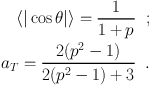
In the most recent analysis Varela et al. (2012) used galaxies from the SDSS DR7 and included disc galaxies with all inclinations via a fit to a thick-disc model using morphological classifications from Galaxy Zoo. The ambiguity in inclination angle was accounted for statistically. Employing a luminosity threshold of Mr = −20.17 + 5 logh, voids with a range of minimum radii between 10 Mpc / h and 18 Mpc / h were identified, with shells for spin measurement between 1 Mpc / h and 10 Mpc / h in thickness. The signals were fitted to the same model as used in the preceding works, but with a different free parameter p which is related to the mean angle and the parameter aT of Equation 30 as follows:
 |
(31) (32) |
Hence p = 1 implies random orientations of galaxies, while p > 1 if galaxy spin is preferentially perpendicular to the vector from void centre to galaxy. Best fits for p and the significance of the alignment signal are shown in Figure 10. For a minimum void radius of 10 Mpc / h and a shell width of 4 Mpc / h, Varela et al. (2012) find no alignment, in agreement with Slosar & White (2009), and corresponding to a constraint aT = −0.003−0.021+0.020 (1σ). Using only voids with radii in excess of ∼ 15 Mpc / h, alignments with aT ≈ −0.5 were found around the 3σ level. Note that aT < 0 indicates a breakdown of the assumptions underlying the model in Equation (30), which states that the spin vector preferentially aligns with the intermediate axis of the tidal shear tensor. Indeed, Varela et al. (2012) found a tendency for parallel alignment with the radius vector of the void, i.e. the major axis of the tidal shear tensor at the surface of the void. This is exactly the opposite finding from Trujillo et al. (2006).
 |
Figure 10. Top: Alignment parameter, p = ⟨ |cosθ| ⟩−1 − 1, as a function of minimum void radius Rmin. See Equation (32) for more details of these quantities. The different lines correspond to the width (SW) in Mpc / h of the shell in which galaxy orientations are measured, in the range 1 to 10 Mpc / h as indicated in the legend. Bottom: As above but showing signal-to-noise ratio (SNR) of the alignment. Negative SNR and p < 1 indicates that the galaxy spin preferentially lies parallel to the line connecting the void centre and the galaxy. © AAS. Reproduced with permission from Varela et al. (2012). |
Hence the observational evidence for galaxy alignments with the surface of voids remains unclear. Varela et al. (2012) stated that the results presented in Trujillo et al. (2006) were selected a posteriori as the configuration with the strongest detection, and re-computed the significance to be less than 2σ. Direct comparison with simulations is hindered by observational selection effects and the difficulty of relating galaxy morphology to halo shape and angular momenta. For instance, Cuesta et al. (2008) found, in N-body simulations, for a similar setup as in the observational studies, aT ≈ 0.04 for spin alignment and aT ≈ −0.17 for minor axis alignment of haloes. Kiessling et al. (2015) provide a detailed discussion of this and other simulation results.
5.4. Galaxy alignments with filaments and sheets
The notion that galaxies are not randomly distributed on the sky but tend to be concentrated in large, elongated structures predates the demonstration of the extragalactic nature of galaxies (Reynolds, 1920). Studies of galaxy position and alignment with respect to the local part of the cosmic web were made from the early 20th century onwards, but results were generally inconclusive and often contradictory. The review by Hu et al. (2006) provides an overview of alignment studies, both early and recent, in the local supercluster.
We first discuss two papers (Lee & Pen, 2002, Lee & Erdogdu, 2007) which, while they do not discuss filaments or sheets explicitly, do look at the alignment of galaxy spin with the shear field eigenvectors, which in turn are very often used to define filaments, as discussed below. Lee & Pen (2002) claimed the first observational evidence for the alignment of galaxy spin with the tidal shear field at the position of the galaxy. They estimated the matter density field from the Wiener-filtered positions of galaxies from the infrared astronomical satellite (IRAS) all-sky survey 5 (Skrutskie et al., 2006). The tidal shear field was then derived via explicit integration and differentiation of the gravitational potential. Galaxy position angle and axis ratio measurements for about 104 spiral galaxies were taken from the photographic plate-based Uppsala General catalogue and its southern counterpart (Nilson, 1973). With these data, Lee & Pen (2002) used the thin-disc approximation to calculate galaxy spin. They rejected a random orientation of galaxy spins at 99.98 % confidence and found aT = 0.17 ± 0.04 (1σ), again using the ansatz in Equation (30).
Lee & Erdogdu (2007) kept the morphology data but included a correction for disc thickness in the calculation of the spin vector and used the 2 Micron All Sky Survey (2MASS) Redshift Survey 6 to determine the tidal field. The 2MASS galaxy positions were expanded on a three-dimensional grid in terms of Fourier-Bessel functions, the tidal field obtained via Fast Fourier Transformation, and then interpolated to the galaxy position. These authors also found a strong detection of spin alignments, obtaining aT = 0.08 ± 0.01 on average, increasing with increasing overdensity. In the context of tidal torque theory, a correlation with aT > 0 means that galaxy spin is aligned with the intermediate axis of the tidal shear tensor (see the argument in Lee & Pen 2001), i.e. their spin vectors tend to be perpendicular to filaments and lie in the plane of sheets.
Jones et al. (2010) selected edge-on galaxies with axis ratio < 0.2 in SDSS DR5 and constructed the matter density field via Delaunay tessellation, using the eigenstructure of the tidal shear tensor to identify filament candidates. These were then inspected visually to select a clean sample of 67 filaments, containing only 69 galaxies with spin measurements. Nonetheless, the authors claimed that the 14 objects among those 67 filaments which were oriented with spins perpendicular to the filament direction (cosθ < 0.2, where θ is the angle between the filament axis and the spin axis) constitute a statistically significant detection of this type of alignment.
Based on SDSS DR8, Tempel et al. (2013) fitted three-dimensional bulge+disc models to the light distribution of galaxies at low redshift (z < 0.2) to infer the spin vector direction. They approximated the filamentary structure by a network of cylinders, defined by elongated overdensities of galaxies. For their full sample of spiral galaxies, no alignment was found, while for a subsample of spirals with Mr < −20.7 the spin axis tended to be parallel to the filament direction. In a sample of flattened early-type galaxies, mostly composed of lenticulars, Tempel et al. (2013) observed a significant alignment of spin perpendicular to the filament axis, which again was stronger for the brightest galaxies. The luminosity dependence could have been due to a physical trend or due to selection effects as, for example, fits to the photometry were more reliable for bright objects. The authors argued that, under the assumption that spiral (S0/elliptical) galaxies mostly live in low-(high-)mass haloes, their findings agree with the established simulation result that massive haloes have their spin aligned orthogonally to filaments, while low-mass haloes show preferentially parallel alignment (e.g. Trowland et al., 2013).
This work was extended by Tempel & Libeskind (2013), who modified the filament-finding algorithm and also included large-scale structure sheets, identified as flattened filaments, i.e. a filament whose detection probability extends into a plane. The authors found no correlation between the spin axis of early-type galaxies (assumed to be the same as the short axis of the galaxy ellipsoid) and the sheet, whereas the spin of spiral galaxies weakly aligns with filaments and tends to avoid pointing away from the filament into the plane of the sheet. These latter signals vanish inside a 200 kpc / h radius around the filament central axis. It is possible that these results are linked to gas infall along the sheets onto the filaments, where angular momentum is generated with a rotation axis along the filament direction.
Zhang et al. (2013) quantified the alignment of the major axes of galaxy images in SDSS DR7 with sheets and filaments. The analysis was based on a catalogue of close to 5 × 10⁵ groups with a minimum estimated halo mass of 1012 M⊙ / h, found using an adaptive halo-based group finder (Yang et al., 2005, Yang et al., 2007). These groups could consist of a single galaxy. Following the method of Wang et al. (2012), the group haloes were used to reconstruct the matter density field via a halo bias model extracted from simulations. Based on this reconstruction, Zhang et al. (2013) identified those groups that resided in a filament or sheet environment via the eigenvalues of the tidal shear tensor at that point (one negative and two positive eigenvalues corresponding to a filament; two negative and one positive eigenvalue corresponding to a sheet), and calculated the angle between the projected major axis of the galaxy and the projected axes of the filament and the sheet normal vector, respectively. Note however, that this study employed the isophotal shapes provided by the SDSS pipeline, which have been flagged as potentially unreliable 7; see Section 1 for more discussion on isophotes and shape measurement.
Figure 11 shows the probability distribution of alignment angles between galaxy and filament (θGF) and galaxy and sheet normal (θGS), for subsamples split into blue/red and central/satellite (centrals are defined as the brightest group galaxies). Generally, galaxies preferentially align with the direction of the filament (small θGF) and lie within the sheet (θGS close to a 90∘ angle). The signals are weak for blue galaxies and highly significant for central (and bright) red galaxies. These dependencies prevail for the alignments of galaxy major axes with the eigenvectors of the tidal tensor. Here, Zhang et al. (2013) find preferentially orthogonal alignment with the largest eigenvector, parallel alignment with the smallest eigenvector and none with the intermediate eigenvector. These results are in good agreement with N-body simulations for red galaxies. The null detection for blue galaxies is somewhat in tension with N-body studies: for example Wang et al. (2011) found significant correlation between the spin axes of dark matter haloes and the eigenvectors of the tidal field. This tension lessens if there is some mismatch between the spin of the overall dark matter halo and that of the galaxy at the centre, which the subsequent study of ??? indicates may be the case.
 |
 |
Figure 11. Left: Renormalised probability distribution of the angle θGF between the projected galaxy major axis direction and the filament axis. For random galaxy orientation a constant value of unity is expected, as indicated by the black dotted line. Error bars are obtained from 100 Monte-Carlo realisations of randomised galaxy orientations. Data are shown for red/blue and central/satellite subsamples, as shown in the legends. Right: Same as on the left, but for the angle θGS between the projected galaxy major axis direction and the sheet normal. © AAS. Reproduced with permission from Zhang et al. (2013). |
|
Zhang et al. (2015) conducted the equivalent study for galaxy spins, reconstructing the three-dimensional direction of the spin vector for galaxies via a simple thick-disc model for galaxies that were classified as spiral by Galaxy Zoo, and as central in their group catalogue. They saw only weak evidence for an alignment with the intermediate axis of the tidal shear tensor (as predicted by tidal torque theory), and therefore for galaxy spins to be preferentially perpendicular to filaments and parallel to the normal of sheets. Comparing their results to N-body simulations, they found better agreement with the observations when calculating the spin only in the inner part of dark matter haloes, i.e. closer to the scales of the bright parts of a galaxy. Since the surfaces of voids and sheets classified via the tidal shear tensor should define similar environments, the results of Zhang et al. (2015) are qualitatively consistent with those of Varela et al. (2012). Note both studies are restricted to low redshifts (z < 0.2 and z < 0.12 respectively), additional studies will be required to increase this baseline.
5.5. Alignments between galaxy groups and clusters
As with galaxy alignments, the alignments of galaxy groups and galaxy clusters with the large-scale structure have received considerable attention. Binggeli, (1982) originally discovered that neighbouring galaxy clusters tend to point towards each other. He found that all pairs of clusters within 30 Mpc of each other (11 out of 30 clusters studied) pointed towards one another, with a misalignment of at most 45∘. West, (1989) showed that this alignment can also be seen for less massive galaxy groups out to similar scales, and Plionis, (1994) found that it decreases with distance and is stronger for clusters residing in the same supercluster.
More recently, Wang et al., (2009) used a large sample of galaxy groups to show that the orientations of groups and their galaxies are strongly correlated. They confirmed the result of West, (1989) that groups tend to point to their nearest neighbours, in addition to showing that group central galaxies point to the nearest group, and that both have preferentially parallel major axes. These effects are strongest for early-type centrals in more massive groups and decline slowly with distance between the groups. Moreover, Paz et al., (2011) showed that this alignment extends to the surrounding large-scale structure, in the sense that groups with masses M ≳ 6 × 10¹³ M⊙ point towards galaxy overdensities in general, and that more massive groups do so more strongly.
In the most recent attempt, Smargon et al., (2012) measured alignments of galaxy cluster pairs out to 100 Mpc / h and z < 0.44 using two galaxy cluster catalogues extracted from SDSS data. The right-hand panels of Figure 12 show their measurements of radial alignment between cluster pairs. They compute these using the “pointing angle”, θp, which is the angle on the sky between the projected cluster major axis and the line connecting one cluster to the other cluster in the pair. A positive correlation is detected out to ∼ 100 Mpc / h. The left-hand panels show a measurement of their common orientations, using the “correlation angle”, θc, that is the angle between the projected major axes of the two clusters. This alignment is marginally detected for pairs separated by less than 20 Mpc / h. The top/bottom panels use different galaxy cluster catalogues, the Adaptive Matched Filament (AMF) (Dong et al., 2008) and maxBCG (Koester et al., 2007) catalogues respectively.
 |
Figure 12. The cluster correlation angle alignment ⟨cos2 θC⟩ (left panels) and the cluster pointing angle alignment ⟨cos2 θp⟩ (right panels), as a function of comoving pair projected separation R in 2D. Note R in this plot is therefore equivalent to the 2D comoving separation that we elsewhere denote as rp. These angles are described in the text. The blue points with error bars are the observational results; the red dashed lines are theoretical predictions from N-body simulations assuming a ΛCDM cosmology (Hopkins et al., 2005), corrected for photometric redshift uncertainties; and the green dotted horizontal lines indicate purely random cluster orientations. The errors between the different bins in R are independent. Top panels: Uses the Adaptive Matched Filament (AMF) catalogue (Dong et al., 2008). Bottom panels: The maxBCG catalogue (Koester et al., 2007). Reproduced with permission from Smargon et al. (2012). |
The observed signals, while significant, are weaker than the predictions from simulations. This discrepancy may be due to idealised assumptions that go into the simulations. Other possibile sources of difference are systematic effects that weaken the observed signal, particularly errors in line-of-sight redshift selection due to the fact that photometric redshifts were used. The photometric redshift errors correspond to typical separations of ∼ 50 Mpc / h along the line-of-sight, leading to contamination from clusters which are really unassociated, thus diluting the signal. Smargon et al., (2012) note that this effect alone cannot explain the full discrepancy; they discuss additional sources of error including centroiding and noise from both the small number of cluster members and clusters that are nearly round.
2 See Joachimi et al. (2015) for details of the history of these observations and the messy nomenclature that resulted. Back.
3 http://www.gama-survey.org/ Back.
4 Note the two works use different conventions for the Hubble constant. Back.
5 http://irsa.ipac.caltech.edu/Missions/iras.html Back.
6 http://www.ipac.caltech.edu/2mass/ Back.
7 https://www.sdss3.org/dr8/algorithms/classify.php#photo_iso Back.