


The IMF has been used as a tool in a broad range of different contexts, as illustrated above. But if the IMF is not universal, then the quantity actually being measured in these different contexts is not necessarily the same. When inferring an IMF based on the integrated light from a galaxy, the quantity being measured is not the same as when inferring an IMF from star counts or luminosity functions. Likewise, when using a cosmic census approach such as the SFH/SMD constraint, the quantity in question is different again.
Such spatial dependence of the IMF has been recognised since the earliest work, with Salpeter (1955) describing the IMF as “the number of stars in [a given] mass range …created in [a given] time interval …per cubic parsec.” The spatial dependence, though, can easily be glossed over, and especially with the idea of a “universal” IMF guiding the thinking, it is easy to conflate IMFs associated with different spatial volumes (star clusters, galaxies) and treat them as the same entity when they may well not be. This can lead to artificial or apparent inconsistencies that may not necessarily be in conflict.
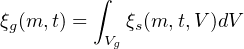
The notion that the IMF within a star forming region is potentially a different quantity than the effective IMF for a galaxy, and different again from the effective IMF for a population of galaxies at a given epoch, is an important foundational concept. Here I define these three quantities as the “stellar IMF” or sIMF (ξs), the “galaxy IMF” or gIMF (ξg), and the “cosmic IMF” or cIMF (ξc) as illustrated in Figure 7. Lower case prefixes and subscripts are chosen here explicitly with the aim of minimising ambiguity between other commonly used variants such as IGIMF (for a galaxy-wide IMF), or CIMF (the cluster IMF for stellar clusters, or “core” IMF for dense gas cores).
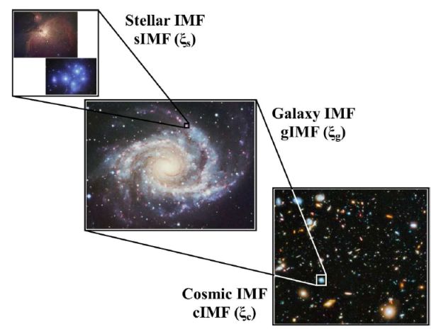 |
Figure 7. A framework to aid in clarifying discussions of the IMF. If the IMF is not universal, then the sIMF, gIMF and cIMF are not necessarily the same, and all may have a time-dependence. Different measurement techniques and observational samples probe these different quantities, and what has been referred to uniformly in published work to date as “the IMF” conflates these distinct properties. This may well contribute to much of the current tension between different IMF estimates in different contexts. |
We can generalise the formalism of the IMF by writing the dependence on time and spatial volume explicitly:
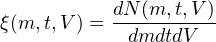 |
(3) |
where dN is the number of stars in mass interval dm created in the time interval dt within the spatial volume dV. In this generalisation it is important to note that the time dependence explicit to ξ allows for the form of the IMF to vary with time. It is different from the time-dependent mass function scaling that arises from a varying SFR, as defined for example by Schmidt (1959).
This approach describes the number of stars of a given mass that have formed up to a given time, for some spatial volume. Over a (short) finite time period and (small) spatial volume this is identically the stellar mass function (not accounting for stellar evolution):
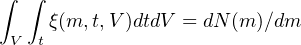 |
(4) |
and corresponds to what might be considered as a “traditional” IMF. This approach eliminates the ambiguity between a nominal, or Platonic ideal, IMF from which real star clusters must be populated, and the actual instantiated mass function, since what is defined here is the real physical quantity of interest, the number of stars formed as a function of mass, time and location. The “universal” IMF scenario can arguably be recovered by asserting that ξ has no temporal or spatial dependence, ξ(m) = dN(m) / dm, but this reopens the issue of accounting for a finite duration for star formation, and the effects of stellar evolution, since such a ξ(m) is in principle never observable (e.g., Kroupa et al., 2013). In contrast, ξ(m, t, V) is directly observable in principle, although in practice doing so may be highly challenging.
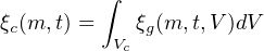
Integrating ξ(m, t, V) over different volumes gives the (time dependent) sIMF, gIMF and cIMF:
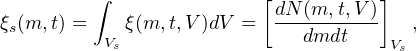 |
(5) |
where Vs is a volume characteristic of a star forming region, for example. Relations for ξg and ξc are analogous.
Clearly there must be a lower limit to the spatial scale or volume over which an IMF is a well-defined quantity, since it makes little sense to attempt to define an IMF at the scale of individual stars, for example. A natural minimum spatial scale is that sufficient to encompass a star cluster, and much of the work on the IMF focuses on the properties of stellar clusters or uses them to probe the IMF (as reviewed by, e.g., Bastian et al., 2010). Also, the volumes referred to here are not specific fixed or comoving volumes in space (although they could be defined as such, in a numerical simulation for example), but refer instead (for convenience) to a particular spatial scale, and which I illustrate through these three representative characteristic scales.
Considering the time dimension too is a revealing mental exercise. The process of star formation is not instantaneous. As stars form within a nascent star cluster there will be different mass functions extant depending on the time step sampled (e.g., Kroupa et al., 2013). There is an extensive literature on the protostellar mass function, explicitly to understand this time dependence in the way that the IMF is generated. McKee & Offner (2010), for example, present a formalism using models for mass accretion by protostars to link the IMF to its progenitor protostellar mass function, extended to the protostellar luminosity function by Offner & McKee (2011). A more recent analytic model for the mass gained by protostars is presented by Myers (2014). Hartmann et al. (2016) review accretion onto pre-main-sequence stars, and their Figure 13 highlights the different stellar mass and luminosity functions expected based on different accretion models.
For a large ensemble of clusters, throughout a galaxy say, each at a different stage in its formation process, the stellar mass function sampled over the full ensemble at a given time step may more closely resemble the mass function expected from a well-defined physical process, such as gravo-turbulent models (e.g., Hennebelle & Chabrier, 2013, Hopkins, 2013b), although the mass function for any individual region may well be rather different, due to the complex feedback effects from stellar evolution during the formation event itself, and the local environment which may be influenced by adjacent regions of star formation or other astrophysical processes.
In this way of thinking, if there is a “universal” physical process that drives star formation, then it is likely to be better sampled on the scales of galaxies (the gIMF) than within individual star forming regions. Extending this idea, and to account for the possibility of variations between galaxies (due to a range of metallicities, star formation environments, and so on), any “universal” physical process might be most accurately sampled through the effective stellar mass function over an entire galaxy population (the cIMF). This leads to the need for the physical processes of star formation to be able to explain potential variations in the stellar mass function from the scale of star clusters to galaxies (which may arise through effects unrelated to the star formation process itself), ultimately converging on a model prediction when sampled over sufficiently large regions. This may be written as ξ (m, t) = ∫V ξ (m, t, V) dV → IMF for V → Vc where Vc is some large volume encompassing one or more galaxies, and “IMF” here is being used to describe the stellar mass function expected from a nominal “universal” physical process.
As an alternative, rather than the sampling of a large spatial volume at a fixed time step, a small volume may be considered over a long period of time to equally ensure that all phases of the physical process of star formation are sampled. This might be summarised as ξ (m, V) = ∫t ξ (m, t, V) dt → IMF for t → tc where tc is large compared to the duration of a star formation event, perhaps capturing multiple such events within the volume V, and “IMF” is used as above. Observationally this is not a practical approach, while the former is, but it may be of value in simulations.
This is another way of considering the arguments posed by Kruijssen & Longmore (2014), as this concept equally applies to the gas clouds from which the stars are forming, and the associated “core” mass functions, or the mass functions of stellar clusters. Any given gas reservoir may not be representative of the full population of star forming gas clouds throughout a galaxy, and only by sampling a sufficient number of them will the statistics of the density distribution be accurately represented.
8.2. Linking mass functions between different spatial scales
With differing stellar mass functions on different spatial scales, a natural question arises regarding how to relate individual mass functions on small scales to those measured on the larger scales, i.e., how to link the sIMF for multiple star forming regions to the gIMF for the galaxy comprising those stars. The IGIMF method (Kroupa & Weidner, 2003, Weidner & Kroupa, 2005, Kroupa et al., 2013) is one approach, which broadly speaking considers a summation of many sIMFs to construct the gIMF. This method assumes that stars form in self-regulated embedded clusters, which follow a relationship between the total mass of a stellar cluster and the mass of its highest mass star. Their sIMFs are therefore empirically constrained by the stellar cluster mass. They can be summed to calculate the gIMF, or the IMF of a region within a galaxy containing multiple stellar clusters, and can lead to a variable gIMF (Yan et al., 2017). This approach allows a gIMF to be calculated given a knowledge of how the sIMF depends on the physical conditions of star formation. The early results using this technique favoured galaxy-wide IMF slopes somewhat steeper at the high mass end than that of the individual star forming regions. Later work incorporating constraints on the variation of the sIMF from Marks et al. (2012) extended this approach to show how flatter IGIMF slopes at the high mass end could be produced in galaxies with high SFRs (Yan et al., 2017).
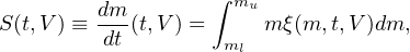
The way that sIMFs themselves arise, or their dependencies on associated astrophysical processes, may differ from the IGIMF assumptions. Some level of variation would seem likely given that star formation happens in a complex multiphase medium, with regions of star formation potentially overlapping, and triggering or suppressing one another in highly non-linear ways, all of which may evolve with time. So the gIMF may not necessarily comprise a sum over a discrete set of identical, or even simply modeled sIMFs. If each such star formation event can be characterised by its own sIMF, though (whether or however it is influenced by, or overlapping with, neighbouring events) we can write
 |
(6) |
where Vg is the volume of the galaxy in question. It is important to distinguish this generalisation from the IGIMF method, since in the current approach each ξs (m, t, V) may arise from different physical dependencies or processes to those assumed in the IGIMF approach.
Likewise, the cIMF may be able to be approximated as a simple sum over gIMFs. Of course, galaxy interactions are an important channel for galaxy evolution, and they are clearly associated in many cases with significant levels of star formation. But assuming for the present argument that stars formed in this mode are a negligible fraction of all stars formed, or alternatively can be accounted for through separate characterisation with their own ξg (m, t, V) we can write
 |
(7) |
where Vc is the cosmic volume being probed.
In this formalism there is no analogue to the process of generating a stellar mass function by “populating” or “drawing from” some underlying IMF, since ξ(m, t, V) here is in effect the stellar mass function itself, incorporating its spatial and temporal variations. Instead, the link to be highlighted is over what spatial or temporal scales this mass function needs to be sampled in order to compare with predictions from various physical models of star formation. In this context questions such as whether the sIMF is drawn from a gIMF, or how to “populate” an sIMF, are poorly posed, and not helpful in developing our understanding of star formation.
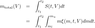
The SFR and total stellar mass are directly linked to the IMF (e.g., Schmidt, 1959), and there is some value in presenting this explicitly. The SFR, S(t, V), is the mass of stars formed in a time interval dt and volume dV:
 |
(8) |
and the total mass in stars ever formed in that volume over some time period t1 to t2 is then:
 |
(9) |
The mass remaining in stars at a time τ is mτ = (1 − R)mtotal, where R is the mass recycled into the interstellar medium (ISM) due to stellar evolutionary processes, and is dependent on the stellar mass distribution. Recycling fractions can be calculated for a given mass distribution if the mass returned to the ISM is known as a function of initial stellar mass (e.g., Renzini & Voli, 1981, Woosley & Weaver, 1995). This is also expected to depend on metallicity.
The value of a “traditional” IMF is largely through the ability to use it as a tool to infer the presence of stellar populations not directly observed. Depending on the techniques being used, observables are often limited either to the high mass (e.g., through Hα, UV, or infrared tracers) or the low mass (e.g., direct star counts, or gravity sensitive spectral features) range of the stellar mass distribution, and accounting for the stellar populations not directly measured is done by invoking an IMF. With an assumed “universal” IMF simply characterised through a well-defined parametric form, such extrapolations are straightforward.
In the general case posed above, a number of simplifying assumptions need to be incorporated in order to regain the utility of the simple “universal” model. The value of the general approach is that these assumptions now become explicit, rather than implicit, defining the form (or absence) of any temporal or spatial variations (which may reflect other underlying physical dependencies). The same parameterisations (incorporating physical dependencies if desired) can be applied as always, using the general formalism, but assumptions about the spatial scale or epoch to which such parameterisations apply become clear. This hopefully enables distinctions to be drawn between stellar mass functions that should not necessarily be compared directly, to avoid artificial inconsistencies. It should also facilitate the exposing of internal contradictions within analyses.
The mass functions as parameterised by, say, Kroupa (2001) and Chabrier (2003a) are not inconsistent with this approach, and they can now be explicitly defined as the integrals over some spatial and temporal scale. So, to the degree that these Milky Way stellar mass functions (IMFMW) correspond to star formation on the scale of star clusters over a period of several Myr, we may write, for example, IMFMW = ∫tt+5 Myr ∫Vs ξ (m, t, V) dV dt, where Vs is the volume sufficient to encompass the star cluster, and 5 Myr is nominally taken as a timescale sufficient to allow the full range of masses for all stars to form. When exploring potential physical dependencies for a stellar mass function, the various observational constraints can be used in this fashion as boundary conditions.
This more general approach can help in setting the context for the broader range of work on the IMF. In particular, by making explicit the potential spatial and temporal dependencies, which are likely a consequence of any underlying physical dependencies, the scales over which certain observational constraints apply also become explicit. It also means that analyses can be clear about the spatial and temporal scales for the stellar mass functions they are using, or making predictions for. For example, the investigation of Blancato et al. (2017) adopts an observed gIMF, which is then implemented as an sIMF in simulations. They find, perhaps not surprisingly given the discussion above, that this does not lead to the observed gIMF being reproduced in the simulated galaxies, concluding that sIMFs need to be more extreme than adopted in order to replicate the observed gIMF.
The approach presented here provides the potential for self-consistent explorations in models and simulations, enables a clearer link between what the models predict and what the observations measure, and avoids conflation between constraints that apply to different physical scales. It provides a framework in which the subtle biases associated with an implicit tendency toward a “universal” IMF are eliminated, allowing for a more critical evaluation of the constraints on potential variations between stellar mass functions, and their link to the underlying physics of star formation.
With these considerations at hand, I now revisit the variety of observational constraints discussed above and position them in this self-consistent framework, in order to re-examine the extent to which the IMF may vary.