


With the extensive sets of measurements, inferences and constraints summarised above, it is helpful in the discussion of the degree of consistency or otherwise to present the results separately for the cIMF (ξc), gIMF (ξg) and sIMF (ξs), to ensure only comparable quantities are being examined. For the Milky Way and nearby galaxies, it may be possible to show these in diagrams representing each of ξg and ξs depending on whether the full galaxy, or star forming regions within it, are shown. This consideration also reveals a distinction between “field star” IMFs and those for stellar clusters, since the “field stars” probe, in a sense, the gIMF, while the stellar clusters probe the sIMF.
It quickly becomes clear when doing this that many published IMF constraints are actually not directly comparable, and that, in fact, there is an extensive range of parameter space to explore in addressing the question of how to characterise the IMF. In the figures below, representative regions are shown for simplicity and by way of illustration, rather than attempting to reproduce individual measurements in detail, especially because in some cases they are not available, although a range of IMF slopes has been given.
In the presentation here I focus on comparisons of IMF shapes as characterised generally by the low and high mass slopes, αl and αh, largely because that is the most common approach taken in the published work. In many cases, though, it may be possible to explain the observed results by a different approach to modifying the IMF shape, such as an increase in mc rather than a more positive (flatter) value of αh, or reducing mu rather than a more negative (steeper) value of αh, for example. Other measures, too, such as αmm, will be important to include in the development of a suite of diagnostic diagrams for constraining the measurement of the IMF. These points should be borne in mind when considering the discussion below.
There are relatively few observations inferring ξc, illustrated in Figure 8, and only αh is typically constrained. A value for αl as steep as Salpeter is ruled out (e.g., Hopkins & Beacom, 2006, Madau & Dickinson, 2014), but most analyses then assume αl = −1.3 (Wilkins et al., 2008b) or αl = −1.5 (Baldry & Glazebrook, 2003, Hopkins & Beacom, 2006) to be consistent with that for the Milky Way. Figure 8 shows the Salpeter slope from Madau & Dickinson (2014), αh=−2.15 from Baldry & Glazebrook (2003), and the evolving high mass slope of Wilkins et al. (2008b). The “paunchy” IMF from Fardal et al. (2007) is not shown, as there are multiple αh values (the slope is different for different mass ranges above m > 0.5 M⊙, see § 6), but these values bracket those shown in Figure 8. The relatively small variation seen in αh demonstrates the potential of the cosmic census approaches in strongly constraining ξc. Already variations in αh for ξc at the 10% level are potentially being discriminated between, and future constraints will be even tighter. It seems fairly clear from this comparison, though, that if the cIMF does evolve, the extent of any evolution needed to resolve the SFH/SMD constraint is relatively mild, and at the level of 10−20% in αh.
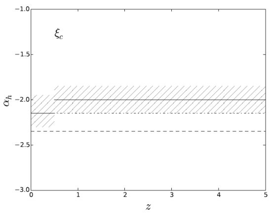 |
Figure 8. The possible variation in αh for ξc from Wilkins et al. (2008b) (solid lines and hatched regions). The dashed line is the Salpeter slope (αh = −2.35), and represents the “universal” IMF from Madau & Dickinson (2014). The dot-dashed line is αh = −2.15 from Baldry & Glazebrook (2003). |
The gIMF has constraints on αh for the star forming population, and on αl for the passive population, but there is no real overlap between the two. The studies constraining αh are not sensitive to αl and vice versa. Figure 9a shows, as an illustration, the range of values for αh from Meurer et al. (2009), Gunawardhana et al. (2011) and Nanayakkara et al. (2017) as a function of redshift, compared with that for the Milky Way (e.g., Kroupa, 2001) and M31 (Weisz et al., 2015). The results of Nanayakkara et al. (2017) at high redshift may well extend to include steeper values, αh < −2.35, although the focus in their discussion is on the possibility of flatter slopes for the extremely high Hα equivalent width systems measured. The dependence of αh on galaxy properties is illustrated in Figure 9b, shown as a function of ΣHα, as inferred from Gunawardhana et al. (2011), Meurer et al. (2009) and Nanayakkara et al. (2017). The relation of αh with ΣSFR from Figure 13 of Gunawardhana et al. (2011) has been converted to one with ΣHα using their SFR conversion factor (their Equation 5). Combining information from Figures 3 and 10b of Meurer et al. (2009), we can infer the range of αh as a function of ΣHα to compare with the results of Gunawardhana et al. (2011) in Figure 9b. The Hα SFR from Figure 21 from Nanayakkara et al. (2017) can be used, with an assumed galaxy size of approximately 3−4 kpc (Allen et al., 2017), and the range of αh inferred from their earlier figures to reconstruct a rough estimate of how their data may populate this relation.
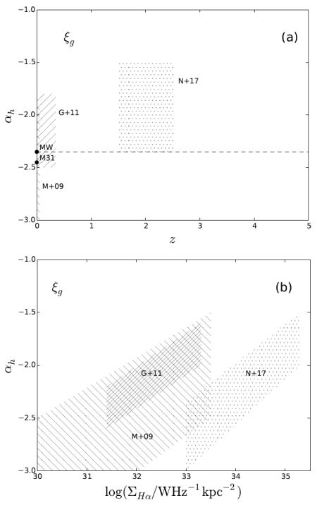 |
Figure 9. (a) The possible variation in αh for ξg from Meurer et al. (2009), Gunawardhana et al. (2011), and Nanayakkara et al. (2017), shown as hatched and dotted regions. The dashed line is the Salpeter slope (αh = −2.35). Values for the Milky Way (MW) and M31 (Weisz et al., 2015) are also shown. Note that the full range of αh is indicated, and the dependencies on sSFR or other physical property are not represented here. (b) The approximate dependence of αh on Hα surface density, inferred from each of Gunawardhana et al. (2011), Meurer et al. (2009) and Nanayakkara et al. (2017). |
The point made by Gunawardhana et al. (2011) is worth reiterating. They state that if an IMF-dependent SFR calibration were used this would have the effect of reducing the range in SFR probed, but would not change their conclusion of an SFR-dependence for αh, since the variation is monotonic and the ordering of the SFRs would not be affected. There is some scope for future work here to develop a self-consistent constraint on αh with SFR-related parameters.
The low mass slope (αl) for ξg is illustrated as a function of redshift in Figure 10. While the galaxies or stars observed in order to infer these measurements are all at very low redshift, the results are shown at illustrative formation times for the stars being analysed, making the coarse assumptions that Milky Way field stars formed 5−10 Gyr ago, while the ages for the passive galaxy stellar populations are taken as approximately 9.5−12.3 Gyr. This approach is taken in order to begin unifying our picture for ξg. So, for example, at z ≈ 2 we have from Nanayakkara et al. (2017) a high mass slope for at least some galaxies up to αh ≈ −1.5 (Figure 9a), with a low mass slope for at least some galaxies of either αl ≈ −1.3 or αl ≲ −2.35. It is interesting to note that there do not seem to be any measurements having intermediate values for the low mass slope of ξg. Observations seem to favour either αl ≳ −1.5 or αl ≲ −2.35. This may echo the bimodality in low mass sIMF shapes implied from the M/L ratios for globular cluster systems from Zaritsky et al. (2014b). They argue that these are consistent with either α = −2.35 for 0.1<m / M⊙ < 100 for the high M/L systems (similar to the results for passive galaxies from, e.g., Conroy & van Dokkum, 2012) and a Milky Way style (Kroupa et al., 1993) IMF (with αl ≈ −1.3) for the low M/L systems.
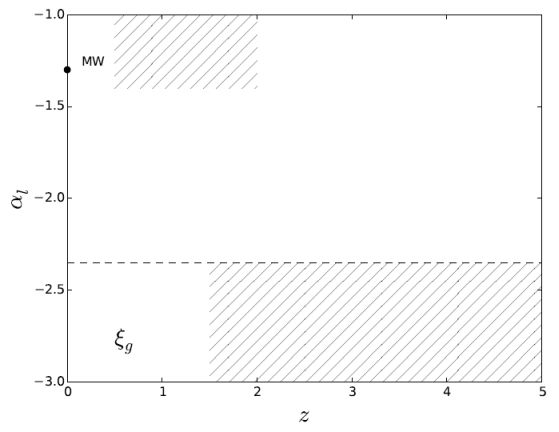 |
Figure 10. The low mass slope of the IMF (αl) as a function of redshift, representative of the formation time of the stars involved. The Kroupa (2001) value for the Milky Way is shown as the data point, and the range of values for αl from Bastian et al. (2010) for Milky Way stars is shown as the upper hatched region, corresponding broadly to formation (lookback) times spanning 5 ≲ t / Gyr ≲ 10. The lower hatched region shows the steep low mass IMF slopes, at formation times approximately 9.5 ≲ t / Gyr ≲ 12.3, for the passive galaxies discussed in § 5.3 above. Note that the broad range of αl for these galaxies is indicated, and potential dependencies on σ or [M/H] are not represented. |
The lensing, kinematic and dynamical constraints on the overall mass normalisation of the gIMF are harder to capture in these kinds of diagrams, as they do not give an explicit constraint on the gIMF shape, and the same mass normalisation can be achieved through various combinations of αl and αh (§ 5.3). In particular, some analyses for passive galaxies use a single power law gIMF to achieve a given mass normalisation, while others constrain αl = −1.3 and achieve the same mass normalisation through inferring a steeper αh. In the latter case, values as steep as αh ≈ −4 (e.g., Martín-Navarro et al., 2015c) are seen for galaxies observed at z ≈ 1 that have formation redshifts around z≈ 2 (contrast with results shown in Figure 9a). As noted by Conroy (2013), to retain a given gIMF mass normalisation, more positive (flatter) values for αh (such as those of Nanayakkara et al., 2017) would imply a need also for more positive (flatter) values of αl, inconsistent with the more negative (steeper) values inferred for passive galaxies from the dwarf-to-giant ratio approach. In other words, the progenitors of low redshift passive galaxies must have had a gIMF different from that observed in situ in high redshift star forming galaxies. This may be a further argument for a bimodality in the gIMF, possibly linked to the stellar M/L ratios for galaxies, that discriminates between spheroid and disk galaxy progenitors.
For the sIMF, ξs, it would be of interest to show αh and αl as a function of age, although here the effects of dynamical as well as stellar evolution would first need to be accounted for (De Marchi et al., 2010). It would also be valuable to explore the sIMF parameters as a function of spatial scale, or total cluster mass, as well as stellar M/L ratio, to assess the potential for a link to ξg. With new telescopes such as the JWST and the GMT enabling the opportunity to explore ξs for more resolved stellar systems within nearby galaxies, it will be valuable to begin quantifying the range of physical parameters currently probed for existing stellar clusters and associations, in order that larger samples spanning a broader range of environments can be put in a common context. In particular, as the sample sizes grow for measuring ξs, there is an opportunity to begin to reduce the sampling errors and discriminate physical effects from sampling effects, in order to establish whether apparent differences between super star clusters, field stars or low SFR regions, and globular clusters are confirmed, and can be attributed to one or more specific physical processes.
The hope is that by discriminating explicitly between ξs, ξg and ξc, and beginning to explore each self-consistently through diagnostic diagrams such as those in Figures 8, 9 and 10, and others that should easily be apparent, clear constraints on any IMF variations should be able to start being quantified.
9.2. Unifying our understanding of the IMF
It is possible to bring this complex suite of observational constraint and inference together by recasting astrophysical questions in this self-consistent approach. Larson (1998) presented a selection of evidence that argued for a “top-heavy” IMF at early times. These included the G-dwarf problem, perhaps now updated as the CEMP star problem, and the evolution of the cosmic luminosity density. The first can now be cast as a constraint on the gIMF, and the second as a constraint on the cIMF (discussed in detail in § 6 above). Importantly, such questions can now be addressed in a quantitative fashion, in order to establish whether any given gIMF, for example, can resolve both the CEMP star constraint and the Kennicutt diagnostic results from Hoversten & Glazebrook (2008), Gunawardhana et al. (2011) and Nanayakkara et al. (2017). Similarly, such gIMFs can easily be assessed to see if they are consistent with the mass normalisation required for the low redshift passive galaxy population. The link between the gIMF and its contributing sIMFs must also be tested, to ensure consistency with the constraints from stellar clusters.
By bringing together the observational constraints in a tractable way, the issue can evolve from individual analyses identifying which IMF form best fits their data, to a set of constraints that must all be met by any successful IMF. This may or may not involve IMF variations, but a strong set of quantitative boundary conditions ensures that any limits on variations can be well measured.
The use of stellar M/L ratios as a unifying property is worth exploring given that it is a quantity that can be applied across a broad range of spatial scales. The similarity shown by Zaritsky et al. (2014b) for the two populations of globular clusters compared to the passive and disk galaxies is tantalising (Figure 2). There may still be a disconnect related to age, though, since the high Υ* globular clusters tend to be those that are young, while the similar Υ* passive galaxies have much older stellar populations. The situation is reversed for the low Υ* globular clusters, which tend to be those with older stellar populations compared to the younger stellar populations with similarly low Υ* in actively star forming disk galaxies. Regardless, there is clearly scope to explore this link further.
It is perhaps worth postulating two broad scenarios at this stage, following from the suggestion above that there may be evidence for a bimodality in forms taken by the gIMF. Scenario 1 is the “bottom heavy” mode, characterised by α = −2.35 over 0.1 < m / M⊙ < 100, and possibly with even steeper αl < −2.35. This mode is that which seems to characterise passive galaxies and their progenitors, high Υ* globular clusters, and possibly low surface brightness or low SFR dSph galaxies or star forming regions. Scenario 2 is the “top heavy” mode, characterised by αh > −2.35 (with αl ≈ −1.3), that appears to be required for high SFR galaxies and star forming regions, and possibly also at high redshift by the cosmic census constraints. It may not be the first time such a model has been proposed, but linking these broad scenarios directly and explicitly with the different sIMF, gIMF, and cIMF constraints will hopefully aid work on the underlying physics of star formation to help clarify which observations (how and in what conditions) the modeled or simulated instantiated mass functions need to be reproduced. A variety of models and simulations already exist that can reproduce such behaviour (see § 7) in at least some circumstances, and the degree to which they self-consistently also reproduce other constraints needs to be tested.
I am hopeful that at this point we can dispense with this question as either misleading or poorly posed. The more relevant question is whether there is a “universal” physical process for star formation. The IMF as a concept is perhaps better presented directly as the evolving and spatially varying stellar mass function explicitly, ξ(m, t, V) (§ 8). Clearly the observed stellar mass functions may vary dramatically between different stellar clusters, associations and galaxies, as a consequence of dynamical and stellar evolution and physical conditions. The stellar mass distribution on the scale of galaxies is not necessarily expected to be the same as that for a star cluster, nor that for a population of galaxies as a whole. There are numerous lines of evidence, summarised above, that the gIMF in particular may show two qualitatively different shapes. In order to assess this further, models and simulations should consider explicitly distinguishing between the IMF on different scales, testing and comparing against observations on appropriate scales. In particular, if there is a “universal” physical process of star formation, that process must lead to the full range of IMF variations seen on the different scales and in the different contexts presented above.
There are many areas where work on understanding the IMF can be developed further, through simulations and observations, some of which are briefly touched on here. These opportunities are qualitatively different for the sIMF, gIMF and cIMF although in all cases, presenting results in terms of IMF independent observables (such as luminosity) as well as derived (IMF dependent) quantities (such as masses and SFRs) is an important aid to clarity.
For the sIMF, especially where stellar systems need to be resolved, new telescopes such as JWST or the GMT will enable significant new breakthroughs. For the cIMF, there is an opportunity to update the review of Madau & Dickinson (2014) by conducting a critical assessment of the many published SFH and SMD measurements, and other cosmic census constraints like the extragalactic background radiation density and supernova rates. This is needed to develop a “gold standard” reference set of observations to serve as the boundary conditions for any cosmic census approach.
As chemical abundance measurements are highly sensitive to the IMF, precision abundance measurements of a large population of stars can be used to improve such constraints. The GALAH survey (De Silva et al., 2015, Martell et al., 2017) is one such project, to deliver precision chemical abundances for a million Milky Way stars, with currently about 0.5 million spectra in hand. Using the technique of “chemical tagging” (Freeman & Bland-Hawthorn, 2002, Bland-Hawthorn & Freeman, 2004, De Silva et al., 2007, Bland-Hawthorn et al., 2010a), the preserved chemical compositions of stars allow the reconstruction of original star-formation events that have long dispersed into the Galaxy background, and possibly even the residual signatures of the first stars in the early universe (Bland-Hawthorn et al., 2010b). In consequence, the large numbers of elemental abundances and large sample size measured by GALAH may enable the most robust measurement yet using this technique of the historical IMF of the Milky Way (G. De Silva, personal communication).
Measurements of the gIMF will continue to be able to draw on a wealth of observational data from existing and upcoming large survey programs, including the large integral field survey SAMI (Croom et al., 2012, Green et al., 2018) and the Taipan galaxy survey (da Cunha et al., 2017) that aims to obtain spectra and redshifts for around 2 million galaxies over the Southern hemisphere. The way the gIMF is measured relies heavily on SPS models, but at present different models are used in different contexts (passive galaxies are analysed one way, star forming galaxies another). There is an opportunity to develop SPS models that can provide the information used in multiple IMF metrics self-consistently. This would allow, for example, the stellar absorption features used in the dwarf-to-giant ratio approach for an old stellar population to be linked directly to the Kennicutt diagnostics for that same stellar population at a younger age, in order to self-consistently assess a passive galaxy population and a star forming galaxy population within a common framework.
Such advances in SPS modeling also need to incorporate the effects of stellar rotation and binarity or multiplicity in stellar systems. There is also an opportunity through new stellar surveys, such as GALAH (De Silva et al., 2015), to extend the range of metallicity and abundances used in stellar evolutionary libraries, on which the SPS models rely. More comprehensively spanning the observed range of stellar properties in this way would reduce the potential that inferred IMF properties might be a consequence of model systematics. This comes, though, at the cost of a greater range of model parameters which may not be observationally well-constrained, and will likely extend these areas of research in their own right.
There is scope to further explore mass-to-light ratio constraints self-consistently with the SPS approaches, by applying both uniformly to a well-defined set of stellar clusters and galaxies. Using both together can break the degeneracy in IMF shape arising from the mass-to-light ratio constraint alone. This approach could potentially lead to a method that links or even unites star cluster constraints with galaxy constraints.
With a field as broad and far-reaching as that of the IMF, there are clearly many more areas in which to pursue improvements in our understanding. Those listed here are just a few that may be valuable to address, directly arising from the discussion and considerations above.