


We now turn to the density profile, phase structure, and kinematics of the CGM. We first present the data that show the various ionization states and velocity distributions of the CGM absorption (Section 4.1). Next, we describe how the absorption line measurements may be translated into physical parameters such as density, temperature, and size in (Section 4.2). We then draw lessons from kinematics (Section 4.3) before considering the physical complexities and challenges inherent in the interpretation of these data (Section 4.4 and Section 4.5).
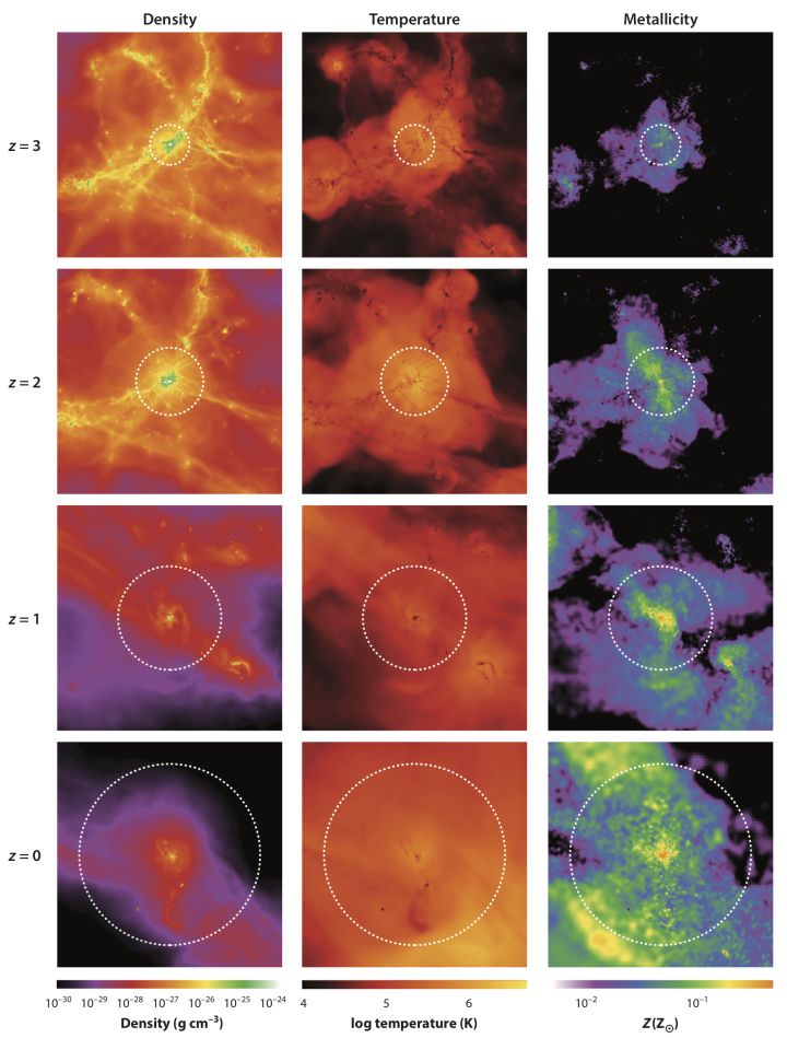 |
Figure 3. These simulated views (from EAGLE, Schaye et al., 2015, Oppenheimer et al., 2016b) of the CGM are more sophisticated but possibly just as uncertain as Figure 1. The four columns render a single galaxy with M⋆ = 2.5 × 10¹⁰M⊙ at z = 0 in density (left), temperature (middle) and metallicity (right). The galaxy is shown at redshifts z = 3, 2, 1, and 0 from top to bottom. The dotted white circle encloses the virial radius at each epoch. |
4.1. The Complex, Multiphase CGM
As a matter of empirical inference, the CGM is “multiphase” in its ionization structure and complex in its dynamics. The ionization structure is seen in Figure 4, which compiles measurements for six diagnostic ions as a function of impact parameter (a proxy for radius). These data indicate a wide range of density and ionization conditions up to a few 105 K with very little interpretation required. Observationally, “multiphase” means many of these metal ions spanning an order of magnitude in ionization potential energy are commonly found within the same “absorber system” occupying a galaxy's halo. An open question in the physics of circumgalactic gas is what this observed mulitphase ionization structure reveals about the small-scale multiphase density, temperature, and metallicity structure of the CGM.
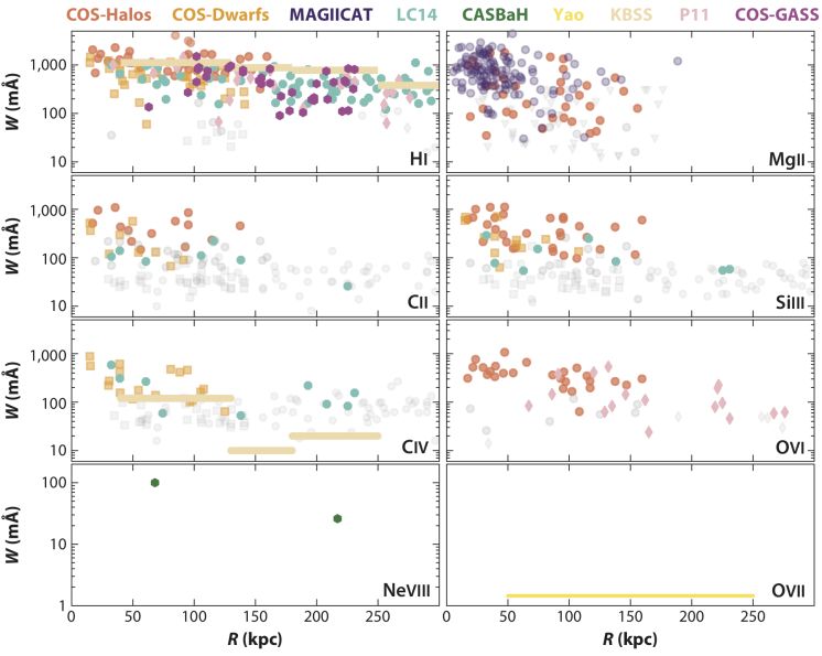 |
Figure 4. A range of ion equivalent width (rest-frame) measurements for a compilation of published surveys. We progress from H i though seven metallic ions of increasing ionization potential. The surveys are COS-Halos Tumlinson et al. (2013), Werk et al. (2013), COS-Dwarfs (Bordoloi et al., 2014b), COS-GASS (Borthakur et al., 2015), MAGIICAT Nielsen et al. (2013), Liang & Chen (2014), the Keck Baryonic Structure Survey (Rudie et al., 2012, Turner et al., 2015), CASBaH (Tripp et al., 2011), Prochaska et al. (2011a), and the X-ray study of Yao et al. (2012) that imposes as stacked upper limit on O vii. |
Over the last 20 years, the practice of using such empirical inputs in analytic arguments to infer the physical state and structure of the diffuse plasma has matured greatly (Mo & Miralda-Escude, 1996, Maller & Bullock, 2004). To produce an extended, multiphase CGM, authors have proposed several scenarios which we categorize as follows: (1) massive inward cooling flows driven by local thermal instabilities (e.g. McCourt et al., 2012); (2) boundary layers between moving cool clouds in a hot atmosphere (e.g. Begelman & Fabian, 1990); and (3) the continual shocking and mixing of diffuse halo gas by galactic outflows (e.g. Fielding et al., 2016, Thompson et al., 2016). We discuss the applicability of some of these analytic models in Section 4.4 and Section 4.5.
Direct evidence for a hot component (logT ≳ 6) in the multiphase CGM comes from diffuse soft X-ray emission (Anderson & Bregman, 2010, Anderson, Bregman & Dai, 2013), and in absorption along QSO sightines (Williams et al., 2005, Gupta et al., 2012) for the Milky Way and external galaxies. Indirect evidence for a hot phase comes from highly ionized metals that correlate with the low-ionization HVCs (Sembach et al., 2003, Fox, Savage & Wakker, 2006, Lehner et al., 2009, Wakker et al., 2012), suggesting boundary layers between a hot medium and the colder HVCs. Milky Way HVCs also show head-tail morphologies indicative of cool clouds moving through a hot medium (e.g., Brüns et al., 2000). Finally, the multiphase CGM is clearly manifested in hydrodynamic simulations, which exhibit a mixture of cool (104 K) and warm-hot (105.5 – 106 K) gas within a galaxy virial radius with a density profile that drops with increased distance from the central host galaxy (e.g., Shen et al., 2013, Stinson et al., 2012, Ford et al., 2013, Suresh et al., 2017, Figure 3). For practical purposes we can regard the outer boundary of the CGM to correspond to Rvir, but there is no empirical reason to believe that any special behavior occurs at that radius; current observations favor trends in column densities that scale with Rvir but do not change in form at that arbitrary boundary.
| Low Ions : IP < 40 eV, T = 104−4.5 K |
| Intermediate Ions : 40 ≳ IP (eV) ≲ 100, T = 104.5 − 5.5 K |
| High Ions : IP ≳ 100 eV, T > 105.5 K |
Evidence for kinematic complexity is revealed as the detected ion species breaking into different “components” with distinct velocities and linewidths. Shown in Figure 5, the various metal ions show significant but varied correspondence in their component structure. The combination of both aligned and misaligned components between ionization states may reflect clouds or streams with density structure or a population of clouds with different ionization states projected together along the line of sight to the same range of observed velocities. Cloud sizes are difficult to constrain in a model independent way, but multiply-lensed images from background quasars (Rauch, Sargent & Barlow, 2001, Rauch & Haehnelt, 2011) prefer 1–10 kiloparsec scales. Fitting Voigt profiles to multi-component absorption yields column density N, Doppler b parameter, and velocity offset v for each component from the galaxy systemic redshift, as well as the total kinematic spread of gas in a halo (but this fitting is subject to issues caused by finite instrumetal resolution). Generally, the kinematic breadth of an absorber system is thought to reflect the influence of the galaxy's gravitational potential, bulk flows, and turbulence in the CGM.
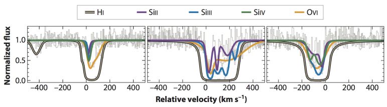 |
Figure 5. A selection of absorption-line data and Voigt profile fits from the COS-Halos survey (Werk et al., 2016), showing a range of metal ions and HI on a common velocity scale with the galaxy at v = 0 km/s on the x-axis. The black outlined beige curve traces H i, the purple Si ii, the blue Si iii, the green Si iv, and the orange shows O vi. |
4.2. From Basic Observables to Physical Properties
We must characterize the ionization states, chemical composition, and density to properly describe the symbiotic relationship with the gas and stars in the central galaxy disk and the CGM. If it were feasible to obtain precise measurements for every ion of every abundant element, in all velocity components, then the gas flows, metallicity, and baryon budget of the multiphase CGM would be well-constrained. However, atomic physics dictates that only a subset of the ionization states of each element lie at accessible wavelengths. Taking oxygen as an example, O i and O vi place strong lines in the far-UV, while O ii – O v lines appear in the extreme-UV (400–800Å). O vii and O viii, arising in hot gas, have strong transitions in the soft X-ray (∼ 20 Å). While it is therefore possible in principle to detect (or limit) every stage of oxygen, this potential has yet to be realized.
| NUV : Near UltraViolet, 2000 ≲ λ ≲ 3400Å |
| FUV : Far UltraViolet, 900 ≲ λ ≲ 2000Å |
| EUV : Extreme UltraViolet, 400 ≲ λ ≲ 900Å |
| X-ray : λ ≲ 30Å |
Figure 6 shows the basic schema for constraining CGM gas properties with these “multiphase” ions. The grey-scale phase diagram renders the properties of all <Rvir gas from a Milky Way mass EAGLE zoom simulation (Oppenheimer et al., 2016b). Accessible ions at each temperature and density are marked with colored squares and dashed lines. This plot is intended to be a useful guide for finding the most likely tracers of a given CGM gas phase. It cannot be used to extract precise temperatures and densities for any given ion since the metal ion positions on this phase diagram are model-dependent. The inset shows the most common strong lines from these species plotted as observed wavelength versus redshift; the rest frame wavelength is where each intercepts z = 0. Practically, FUV lines are available at z < 1 with Hubble and z > 2 from the ground, the EUV lines can be reached at z ≳ 0.5−1 with Hubble (λobs ≳ 1100 Å), and the X-ray lines can currently only be detected toward the small number of bright QSOs and blazars with reach of the sensitivity of Chandra and XMM. As a result, most CGM measurements rely on heterogeneous ion sets — several low ions from C, N, Si, and Mg, a few intermediate ions from C and Si, and a high ion or two from Ne and O. Therefore, the gas density and temperature can only be understood in the context of a model for its ionization state (and abundance patterns).
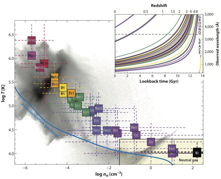 |
Figure 6. Metal absorption lines (ions) of the CGM from Mg i to O viii having 19 < λrest < 6000 Å shown on a phase (T - nh) diagram within Rvir of the z = 0 EAGLE simulation shown in Figure 2. The points are colored according to ionization state, ranging from neutral (I; black) to highly ionized (X; magenta). The position of each point is set on each axis where its ionization fraction peaks in CIE (temperature axis) and a standard PIE model (density axis) (Gnat & Sternberg, 2007b, Oppenheimer & Schaye, 2013a); the range bars show the T and n range over which each species has an ionization fraction over half its maximum value (i.e., the FWHM). Complete line lists are available in Morton (2003). |
Many assumptions are necessary to make progress toward physical models of the CGM. The two most generic classes of models are PIE and CIE. Generally, low and intermediate ions can be accommodated within PIE models, while high ions require CIE models. Species at intermediate ionization potentials, such as C iv and O vi, will sometimes show a preference for one or the other or have contributions from both. These two classes of model are not mutually exclusive: a gas that is collisionally ionized may have the ion ratios further affected by incident radiation, and there are numerous possible departures from equilibrium that further complicate modeling (e.g. Gnat & Sternberg, 2007b). Generally, having access to more metal ion tracers means one is able to place more refined constraints on the models, while results from models with fewer ions are more model-dependent.
| CIE : Collisional Ionization Equilibrium |
| PIE : PhotoIonization Equilibrium |
| EUVB : Extragalactic UltraViolet Background |
Radiative transfer models like Cloudy (Ferland et al., 2013) are used to build PIE models (e.g. Bergeron & Stasińska, 1986, Prochaska et al., 2004, Lehnert et al., 2013, Werk et al., 2014, Turner et al., 2015), which are parametrized by density nh, or equivalently the ionization parameter logU ≡ Φ/nh c, the observed neutral gas column density NHI, and a gas-phase metallicity, log [Z/H]. Here, Φ is the number of photons at the Lyman edge (i.e., the number ionizing photons), set by the assumed incident radiation field with a given flux of ionizing photons. Besides ionization and thermal equilibrium, another major underlying assumption of photoionization modeling is that the included metal ions arise from a single gas phase with the same origin (i.e., are co-spatial). The single cloud, single density approximation for PIE modeling of low-ions leads to uncertain “cloud” sizes, determined by Nh/nh ranging from 0.1–100 kpc (Stocke et al., 2013, Werk et al., 2014). In response, some models have begun to explore internal cloud density structure (Stern et al., 2016) or local sources of radiation (e.g. star-formation in the galaxy, the hot ISM, Fox et al., 2005, Werk et al., 2016). PIE models generally fail for highly-ionized metal species like O vi, sometimes C iv, and certainly for X-ray ions. For those we turn to CIE, where temperature controls the ionization fractions and a metallicity must be assumed or constrained to derive total hydrogen column Nh.
Beyond PIE and CIE, there are non-equilibrium ionization mechanisms that may reproduce the intermediate- and high-ion states that generally fail for PIE (e.g. C iv, N v, O vi). These models include: (1) radiative cooling flows that introduce gas dynamics and self-photoionization to CI models (Edgar & Chevalier, 1986, Benjamin, 1994, Wakker et al., 2012), (2) turbulent mixing layers, in which cool clouds develop skins of warm gas in Kelvin-Helmholtz instabilities (Begelman & Fabian, 1990, Slavin, Shull & Begelman, 1993, Kwak & Shelton, 2010), (3) conductive interfaces, in which cool clouds evaporate and hot gas condenses in the surface layer where electron collisions transport heat across the boundary (Gnat, Sternberg & McKee, 2010, Armillotta et al., 2016), and (4) ionized gas behind radiative shocks, perhaps produced by strong galactic winds (Dopita & Sutherland, 1996, Heckman et al., 2002, Allen et al., 2008, Gnat & Sternberg, 2009). These models all modify the column density ratios given by pure CIE, but do not change the basic conclusion that gas bearing these ionic species must be highly ionized, i.e. with a neutral fraction ≪ 1%. These large and unavoidable ionization corrections, when applied to H i column densities of logNHI ∼ 15–18, entail surface densities and total masses that are significant for the galactic budgets (Section 5). It is likely that combinations of PIE and CIE into these more complex models are more accurate descriptions of Nature than either basic process considered in isolation.
4.3. Line Profiles and Gas Kinematics
Linewidths, given by the Doppler b parameter, illuminate the CGM temperature structure and gas dynamics. The gas temperature, T, and any internal non-thermal motions are captured in the following parameterization: b2 = (2kT / mi) + bnt2, for a species with atomic mass mi. When the low and high ions are assessed via Voigt profile fitting, the low ions are usually consistent with gas temperatures < 105 K, with a contribution from non-thermal broadening (< 20 km s−1, Tumlinson et al., 2013, Churchill et al., 2015, Werk et al., 2016). “Broad Lyman alpha” (BLA; b ≳ 100 km s−1) and Ne viii systems have been detected in QSO spectra at high S/N that directly probe gas at logT ∼ 5.7 (Narayanan et al., 2011, Savage, Lehner & Narayanan, 2011, Tripp et al., 2011, Meiring et al., 2013). These UV absorption surveys indicate that the CGM contains a mixture of photoionized and/or collisionally ionized gas in a low-density medium at 104 - 105.5 K (e.g., Adelberger et al., 2003, Richter et al., 2004, Fox et al., 2005, Narayanan et al., 2010, Matejek & Simcoe, 2012, Stocke et al., 2013, Werk et al., 2013, Savage et al., 2014, Lehner et al., 2014, Turner et al., 2015).
The velocity dispersion and number of components reveals the kinematic substructure of the CGM. Most significantly, gas near low-z galaxies across the full range of log M⋆ = 8.5–11.5 show the projected line-of-sight velocity spreads that are less than the inferred halo escape velocity, even accounting for velocity projection. Thus most of the detected CGM absorption is consistent with being bound to the host galaxy, with implications for outflows and recycling (Section 7). This is true for all the observed species from H i (Tumlinson et al., 2013) to Mg ii (Bergeron & Boissé, 1991, Nielsen et al., 2015, Johnson, Chen & Mulchaey, 2015b) to O vi (Tumlinson et al., 2011, Mathes et al., 2014). The strongest absorption seen in H i and low ions are heavily concentrated within ± 100 km s−1. For low ionization gas, internal turbulent / non-thermal motions are bnt ∼ 20 km s−1, while for high ionization gas the non-thermal/turbulent contributions to the line widths are 50–75 km s−1 (Werk et al., 2016, Faerman, Sternberg & McKee, 2017). Similar total linewidths are seen in the z > 2 KODIAQ sample, possibly indicating similar physical origins at different epochs Lehner et al. (2014).
Mis-alignments of the high and low-ion absorption profiles in velocity space may indicate that the gas phases bearing high and low-ions are not co-spatial and thus that the gas is multiphase (e.g. Fox et al., 2013). Some systems, however, show close alignment between low and high ionization gas (Tripp et al., 2011) in a fashion that suggests each detected cloud is itself multiphase, perhaps in a low-ion cloud / high ion skin configuration. Heckman et al. (2002) and others (e.g. Grimes et al., 2009, Bordoloi, Heckman & Norman, 2016) have argued that the relationship between O vi column density and absorption-line width for a wide range of physically diverse environments indicates a generic origin of O vi in collisionally-ionized gas. However, the relationship exhibits considerable scatter, is impacted significantly by blending of multiple unresolved components (at least at the moderate R ∼ 20,000 resolution of COS), and may arise from other physical scenarios such as turbulent mixing (e.g. Tripp et al., 2008, Lehner et al., 2014). Generally, high-ions like O vi in the CGM exhibit systematically broader line widths than low and intermediate ions (e.g. Werk et al., 2016). Though complex and varied, absorber kinematics may provide important observational constraints on both ionization and hydrodynamic modeling, but new methods of analysis and new statistical tools will be required to realize their full potential.
4.4. Challenges in Characterizing the Multiphase CGM
Ionization modeling is limited by what might be considered “sub-grid” processes that investigators must cope with to get from line measurements to useful constraints on models. The most basic of these arise in the data themselves. CGM absorption observations are generally not photon-noise limited, but line saturation is a major issue particularly for the most commonly detected species. Only lower limits can be derived from the equivalent widths of saturated lines; line profile fitting helps where the saturation is not too severe. Reliable columns of the crucial H i ion are often challenging except where the Lyman limit is available. Moreover, the blending of narrow components with small velocity offsets in data with finite spatial resolution make all line measurements somewhat ambiguous. It is often necessary to model an entire line profile as a single nominal cloud, though sometimes the ionization state can be constrained on a component-by-component basis.
There is often ambiguity about whether to adopt PIE, CIE, or combination non-equilibrium models. These issues are compounded by uncertainties in the additional model inputs. These include the relative elemental abundances, which need not be solar but are usually assumed to be. The EUVB is a particular problem as it may be uncertain especially at low redshift (Kollmeier et al., 2014), introducing up to an order of magnitude systematic error into some ionic abundances (Oppenheimer & Schaye, 2013b).
Though O vi is among the strongest and most frequently detected CGM metal absorption line, it amply demonstrates the problems encountered in precisely constraining the exact physical origins of ionized gas. For example, absorption-line studies in high-resolution and high-S/N QSO spectra and complementary studies of HVCs around the MW show that the ionization mechanisms of O vi are both varied and complex over a wide range of environments (e.g. Sembach et al., 2004, Tripp et al., 2008, Savage et al., 2014). Ionic column density ratios and line profiles sometimes support a common photoionized origin for O vi, N v, and low-ion gas (e.g. Muzahid et al., 2015), while other systems require O vi to be collisionally ionized in a ∼105.5 K plasma (e.g. Tumlinson et al., 2005, Fox et al., 2009, Tripp et al., 2011, Wakker et al., 2012, Narayanan et al., 2011, Meiring et al., 2013, Turner et al., 2016). Often, the multiple components for a single absorber show both narrow and broad absorption lines consistent with both scenarios.
All these thorny issues with ionization modeling highlight the difficultly of getting at the detailed “sub-grid” physics of a complex, dynamic, ionized medium. We should maintain a cautious posture toward conclusions that depend sensitively on exact ionization states. Much of the detailed physics is still at scales that we cannot yet resolve. Nevertheless, in Section 5 we will see what we can learn by simplifying the situation to the most basic classes of models and proceeding from there.
The “Galactic Corona” began with Spitzer's insight that cold clouds could be confined by a hot surrounding medium. This model has matured over the years into a strong line of theoretical research focused on the detailed physics of how the thermal, hydrodynamic, and ionization state of CGM gas evolves in dark matter halos. Placing multiphase gas into the context of the dark matter halo, Maller & Bullock (2004) suggested cold clouds cooled out of thermal instabilities in a hot medium, while maintaining rough pressure equilibrium (though see Binney, Nipoti & Fraternali (2009) for a counterpoint). Accretion may also be seeded by gas ejected from the disk, as in the “galactic fountain” or “precipitation” model (Fraternali & Binney, 2008, Voit et al., 2015b, e.g.,). These scenarios start with very simple assumptions–such as hydrostatic hot halos, diffuse clouds in photoionization equilibrium, or particular radial entropy profiles. These simplifying assumptions are necessary because we do not know the large-scale pjhysical state of the CGM as a whole. Photoionization modeling of the low-ionization CGM using only the EUVB (Haardt & Madau, 2001) strongly disfavors hydrostatic equilibrium with hot gas at Tvir (Werk et al., 2014); the cool and hot phases appear to have similar densities, rather than similar pressures. Furthermore, if O vi-traced gas follows a hydrostatic profile at the temperature where its ionization fraction peaks, T ∼ 105.5 K, then its column density profile would be significantly steeper than observed (Tumlinson et al., 2011). There may be other means of supporting this gas, such as turbulence (Fielding et al., 2016), cosmic rays (Salem, Bryan & Corlies, 2016), or magnetic fields.
Adding to the uncertain physical conditions in the CGM is the fact that O vi likely represents a massive reservoir of warm gas (Section 5.2.3). Such a massive reservoir is apparently at odds with the short cooling times for O vi given by typical CI models; these timescales are often much shorter than the dynamical time, on the order of ≲ 108 yr. Yet, the short cooling times for O vi are in fact characteristic of many models for the multiphase CGM. In many formulations, the cooler low-ion traced gas precipitates out of the warmer O vi-traced phase, owing to thermal instabilities (Shapiro & Field, 1976, McCourt et al., 2012, Voit et al., 2015b, Thompson et al., 2016; see also Wang, 1995), while the O vi-traced gas may be continually replenished by a hot galactic outflow. In a similar vein, the O vi-traced warm gas could be cooling isochorically out of a hotter halo (e.g. Edgar & Chevalier, 1986, Faerman, Sternberg & McKee, 2017) but overcome its short expected lifetime by extra energy injection from star formation or AGN.
Fully understanding the broader context and origin of the multiphase CGM will require more than microphysical and phenomenological models alone can offer. Cosmological hydrodynamic simulations with self-consistent cosmic accretion and multiphase outflows are key to deciphering the panoply of observed absorption lines (Section 7). Moreover, much of the microphysics proposed as a natural source or maintainer of multiphase gas (e.g., thermal instabilities and turbulence) requires resolutions much higher than can be achieved by simulations that must simultaneously model a the enormous dynamic range required for galactic assembly. Yet essentially all cosmological hydrodynamic simulations do produce a multiphase CGM (see, e.g., Figure 3). In general, the combination of the simulated density and temperature profiles of the CGM results in different ions preferentially residing at different galactocentric radii, with low-ions preferring the denser, cooler inner CGM and higher ions filling the lower density, hotter outer CGM (Hummels et al., 2013, Ford et al., 2014, Suresh et al., 2015; see also Stern et al. (2016)). Yet inhomogeneous mixing of the different gas phases complicates predictions for gas cooling rates and the small-scale metal mixing which depend crucially on the unknown diffusion coefficient (Schaye, Carswell & Kim, 2007).
Hydrodynamic simulations may be compared directly to observations via synthetic spectra, potentially helping to disentangle the degeneracy between physical space and observed velocity space. Constructing these synthetic spectra, however, faces many of the same challenges as modeling the ionization states of the observed gas: while the density, temperature, and metallicity of the simulated gas may be known, the EUVB and ionization mechanism must still be assumed in order to calculate ionization states (see, e.g., Hummels, Smith & Silvia (2016)). Most simulations rely on the same radiative transfer codes (e.g., Cloudy, Ferland et al., 2013) that observational analyses do, though non-equilibrium chemistry and cooling are being included as computation power increases (Oppenheimer & Schaye, 2013a, Silvia, 2013). If these assumptions are incorrect, comparisons of derived results (such as masses) rather than observables (such as column densities) may lead to simulations getting the “right answer” for the wrong reasons.