5. THE BARYONIC MASS DISTRIBUTION OF THE CGM

5.1. The Missing Baryons Budget

Empirically constraining the total CGM mass as a function of stellar and/or halo mass is essential to quantifying models of galactic fueling and feedback. Under the condition Ω_b / Ω_m = 0.16 (Planck Collaboration et al., 2013), the total baryonic budget of sub-L^* to super-L^* galaxies spans two orders of magnitude, ranging from 10^10.3 − 10^12.3 M_⊙. Although the stars and ISM for super-L^* galaxies are similar fractions of the total (∼ 5%), the absolute amount of mass that must be found is around 100× larger for sub-L^* galaxies and 10× larger for L^* galaxies. How much of this 80–90% missing mass is in the CGM? We organize this subsection by temperature, and review the observations, assumptions, and uncertainties in each calculation, using Figures 7 and 8 to synthesize current results. We note that a recent review by Bland-Hawthorn & Gerhard (2016) performed a similar radially-varying mass-budget compilation for the Milky Way and its halo and incorporates some of these same results.

The baryon census as presented here relies on the assumption that galaxies fall along well-defined scaling relations of ISM and CGM gas mass as a function of stellar mass, and that the scatter in these scaling relations is uncorrelated. We caution that there is tentative evidence that this is not necessarily the case: COS-GASS has shown galaxies with more cold gas in their ISM have more cold gas in their CGM (Borthakur et al., 2015). While the correlation between CGM and ISM exhibits a high degree of scatter, likely from patchiness in the CGM, it exists at > 99.5% confidence, and stacked Lyα profiles for low and high ISM masses clearly show the effect. The large-scale environment and gaseous interstellar content are difficult to explicitly account for in overall baryon budgets, and may account for some of the scatter in the various estimates. For example, Burchett et al. (2015) find that the detection of C iv around galaxies with M_⋆ > 10^9.5M_⊙ drops significantly for galaxies in high-density regions (see also, Johnson, Chen & Mulchaey, 2015a). Future work should control for these properties.

5.2. CGM Masses by Phase

5.2.1. Cold Gas, T < 10⁴ K. Cold-gas tracers consist of neutral and low ions like H i, Na i, Ca ii, and dust. This is material that may have cooled from hotter phases that experienced thermal instability, or may arise in clouds entrained in multiphase outflows. Putman, Peek & Joung (2012b) estimated the total cold gas mass traced by HVCs in the Milky Way halo to be M = 2.6 × 10⁷ M_⊙ (including only HVCs detected via 21 cm emission, and excluding the Magellanic Stream system). The Magellanic Stream provides an additional contribution of ∼ 3 × 10⁸ M_⊙, but it cannot be assumed to be a generic feature of galaxies. Thus, the total contribution from cold gas is M ≲ 10⁹ M_⊙ even if the ISM of the Clouds are included, making up less than 1% of the missing baryons for a Milky-Way like halo. We further note that while dust masses have been estimated from stacks of reddened background QSOs (Ménard et al., 2010) and galaxies as “standard crayons” (Peek, Ménard & Corrales, 2015) indicating values comparable to the dust in the ISM of these galaxies (see Section 6.3), both ISM and and CGM dust are at most only ∼1% of the missing halo baryons. Finally, using stacked optical spectra from SDSS, Zhu et al. (2013) derived a column density profile for gas bearing Ca ii H and K around ∼ L^* galaxies. For the purposes of Figure 5 we have converted this to a mass density profile, conservatively assuming that the calcium is entirely in Ca ii and Z = Z_⊙. The total mass for Ca ii itself is 5000 M_⊙, and when we scale to Z = Z_⊙ we derive M = 2 × 10⁸ M_⊙for the cold component, again ∼ 1% or less of the baryons budgets.

5.2.2. UV Absorption Lines and the Cool 10⁴⁻⁵ K CGM. The mass of the cool CGM (∼ 10⁴⁻⁵ K) is perhaps the best constrained of all the phases at low redshift, owing to the rich set of UV lines in this temperature range. Prior to COS, estimate for this phase were based on single ions with very simple ionization and metallicity corrections to arrive at rough estimates. Prochaska et al. (2011b) estimated M_cool ≈ 3 × 10¹⁰ M_⊙ for all galaxies from 0.01 L^* to L^*, assuming a constant N_h = 10¹⁹ cm⁻² out to 300 kpc. Using a “blind” sample of Mg ii absorbers, Chen et al. (2010) estimated M_cool ≈ 6 × 10⁹ M_⊙ for the Mg ii-bearing clouds alone. The former estimate simply took a characteristic ionization correction, while the latter counted velocity components as clouds and converted from a metal column density to N_h using a metallicity, because neither study had the multiphase diagnostic line sets that could be used to self-consistently constrain gas density and metallicity. Both L^* and super-L^* galaxies have provided the most reliable constraints, mainly due to their relative ease of detection in photometric and spectroscopic surveys at z < 0.5 (Chen & Mulchaey, 2009, Prochaska et al., 2011b, Werk et al., 2012, Stocke et al., 2013).

With COS, it became practical to build statistically significant samples of absorbers that cover a broader range of ions. These estimates still rely on photoionization modeling, carried out under the standard assumption that the low-ions and H i trace cool (T < 10⁵ K) gas and the primary source of ionizing radiation is the extragalactic UV background (UVB). Using the COS-Halos survey, Werk et al. (2014) addressed the mass density profile and total mass for L ≈ L^* galaxies with PIE models that derive self-consistent n_h and Z using a range of adjacent ionization states of low-ion absorption lines (primarily C ii, C iii, Si ii, Si iii, N ii, and N iii). The resulting surface density profile appears in Figures 7, and yields M_cool = 6.5 × 10¹⁰ M_⊙ for L^* galaxies out to R_vir. Using the same COS-Halos sample with new COS spectra covering the Lyman limit, and taking a non-parametric approach with a robust treatment of uncertainties, Prochaska et al. (2017) recently refined the cool CGM mass estimate to be 9.2 ± 4.3 × 10¹⁰ M_⊙ out to 160 kpc. Stocke et al. (2013) used the complementary approach of estimating of individual cloud sizes and masses, along with their average volume filling factor, for galaxies in three luminosity bins (< 0.1 L^*, 0.1−1 L^*, and L > L^*). They find volume filling factors that range from 3-5% for their modeled clouds, with length scales (N_h / n_h) ranging from 0.1–30 kpc, totaling logM_cool = 7.8 − 8.3, 9.5 − 9.9, and 10 − 10.4, respectively. Finally, Stern et al. (2016) determine the total mass in the cool (and possibly warm CGM) of 1.3 ± 0.4 × 10¹⁰M_⊙ for L^* galaxies given their “universal” cloud density profile. In this phenomenological model each ion occupies a shell of a given n and T such that the fraction of gas in that particular ionization state is maximized. Thus, this calculation represents a conservative minimum of baryons that must be present. These ranges are shown in Figure 8.

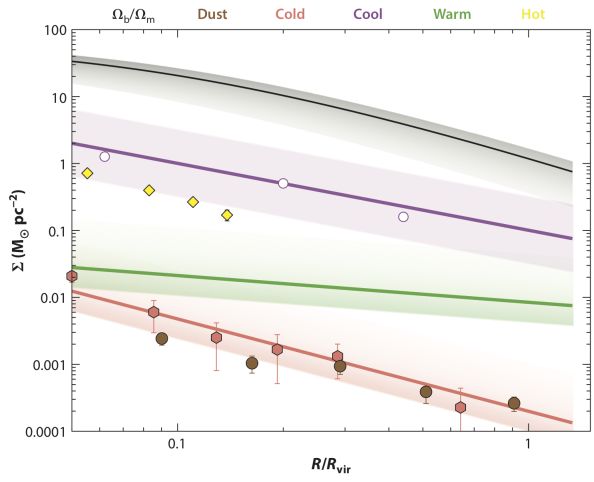Figure 7. A synthesis of CGM mass density results for “cold gas” (pink, Zhu & Ménard, 2013b), “cool gas” (purple, Werk et al., 2014), “warm gas” traced by O vi (green, Tumlinson et al., 2011, Peeples et al., 2014) X-ray emitting gas (yellow, NGC 1961, Anderson, Churazov & Bregman, 2016), and dust (brown, Ménard et al., 2010). An NFW profile for MDM = 2 × 1012 M⊙ is at the top in black.

For super-L^* galaxies, Zhu et al. (2014) use stacking techniques to estimate the correlation function between luminous red galaxies with a mean stellar mass of 10^11.5 M_⊙ and cool gas traced by Mg ii absorption in SDSS data for ∼ 850,000 galaxies with 0.4 < z < 0.75. The cool CGM around massive galaxies calculated in this way appears to completely close the CGM baryon budget for super-L^* galaxies, at 17% of the total halo mass. The assumptions for metallicity and ionization corrections, however, make it uncertain.

5.2.3. UV Absorption Lines and the Warm 10⁵⁻⁶ K CGM. In Figure 6, it appears as though ions like C iv, N v, O vi, and Ne vii trace the warm CGM at T ≈ 10⁵⁻⁶ K. However, this temperature range in particular is burdened by significant uncertainty in the precise ionization mechanism responsible for its purported ionic tracers (see Section 4.4). If high-ions are partially photoionized, O vi for example, may trace a non-negligible fraction of T < 10⁵ K gas that has already been counted toward the total baryon census in the previous section. For gas traced by O vi, Werk et al. (2016) point out that typical photoionization models like those used for the low-ions have difficulty accounting for the total column of O vi and column density ratios of N v / O vi without the need for path lengths in excess of 100 kpc. However, significant additional ionizing radiation at ∼ 100 eV may reduce this requirement.

In general, CIE models require a very narrow range of temperature to reproduce the O vi observations, T = 10^5.3−5.6 K (Tumlinson et al., 2011, Werk et al., 2016). Furthermore, the kinematics of O vi relative to the low-ions, in particular large b values, seem to naturally support the idea that the O vi is in a hotter phase (Tripp et al., 2011, Muzahid et al., 2012; see also Tripp et al., 2001, Stern et al., 2016). Tumlinson et al. (2011) found that O vi traces a warm CGM component that contributes > 2 × 10⁹ M_⊙ of gas to the L^* baryon budget. This mass estimate is strictly a lower limit due to the conservative assumptions adopted: (1) solar metallicity; (2) the maximum fraction of oxygen in O vi allowed by CIE models, 0.2, and (3) the CGM sharply ends at 150 kpc. We adopt logM_warm = 10.0 in Figure 8 for the COS-Halos galaxies (see also Faerman, Sternberg & McKee 2017).

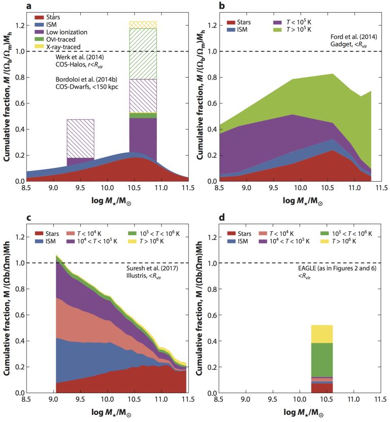Figure 8. Upper left: An accounting of CGM baryon budgets for all physical phases. The solid bars show the minimum values, while the hatched regions show the maximal values. The other three panels show simulated baryon budgets from Ford et al. (2014) in the upper-right, Illustris (Suresh et al., 2017) in the bottom left, and in the bottom right, the EAGLE halo shown in Figures 2 and 6 (Schaye et al., 2015, Oppenheimer et al., 2016b).

For sub-L^* galaxies, Bordoloi et al. (2014b) estimate M_warm using C iv. As these galaxies are at z < 0.1, the COS spectra do not cover the full range of Lyman series lines and ions available at z > 0.1, hindering detailed ionization modeling. COS only covers O vi at z > 0.2, where it is difficult to assemble statistically significant samples of confirmed sub-L^* galaxies, so an O vi-based mass estimate for low-mass galaxies is not currently possible. With these caveats in mind, assuming a limiting ionization fraction for C iv, Bordoloi et al. derive logM_warm = 9.5, if the gas typically has solar metallicity. For gas with lower metallicity, e.g., 0.1 solar, the value is 10 times higher and rather closer to baryonic closure for sub-L^* galaxies (Figure 8). We caution that for C iv, detailed photoionization often places C iv with low-ionization state gas rather than with high-ionization state gas (e.g., Narayanan et al., 2011). Thus, the C iv-derived mass for sub-L^* galaxies is highly uncertain without detections of additional ionization states.

One of the most surprising results to emerge from Tumlinson et al. (2011) is that O vi appears to be absent around the non–star-forming, more massive galaxies in the COS-Halos sample. Thus, there is tentative evidence that ∼ 10^5.5 K gas is not a major component of the CGM of super-L^* galaxies, which may be a result of massive galaxies having generally hotter halos or non-equilibrium cooling (Oppenheimer et al., 2016b). Thus, we do not have a good observational constraint for the warm CGM baryonic content for super-L^* galaxies. The extreme-UV ion Ne viii redshifts into the COS band at z > 0.5, where a few detections (Tripp et al., 2011, Meiring et al., 2013) hint that it may be present in halos out to 100–200 kpc. However, the number of absorbers associated with particular galaxies is not yet sufficient to include it in mass estimates for the warm phase.

5.2.4. The Hot T > 10⁶ K Phase. Hot gas at the virial temperature (T_vir = GM_halo m_p / k R_vir) is a long-standing prediction. For M_halo ≳ 10¹²M_⊙, the temperature should be T ≳ 10⁶ K, and observable at X-ray wavelengths, although there are extreme-UV tracers such as Mg x and Si xii that have yet to yield positive detections (Figure 4). Only a few very luminous spirals and ellipticals have had their halos detected (Anderson & Bregman, 2011, Dai et al., 2012, Bogdán et al., 2013, Walker, Bagchi & Fabian, 2015, Anderson, Churazov & Bregman, 2016), and independent constraints the temperature, density, and metallicity profiles from soft X-ray spectroscopy is rarer still. Thus the fraction of baryons residing in the hot phase, and its dependence on stellar and or halo mass, are not yet determined.

Three sets of constraints are relevant: the Milky Way, individual external galaxies, and stacked samples of external galaxies. Anderson & Bregman (2010) addressed directly the problem of whether hot gas could close the baryon budget for the Milky Way. From indirect constraints such as pulsar dispersion measures toward the LMC, cold gas cloud morphology, and the diffuse X-ray background, they limited the hot gas mass to M ≲ 0.5−1.5 × 10¹⁰ M_⊙, or only 2-5% of the missing mass. The choice of an NFW profile for the hot gas is a key assumption: if the density profile is assumed to be flatter (β ∼ 0.5), the mass can be 3-5 times higher, but still only 6-13% of the missing baryons. The Gupta et al. (2012) claims that the baryon budget is closed for the Milky Way, based on the assumption of an isothermal, uniform density medium, have been questioned by evidence that the gas is neither isothermal nor of uniform density (Wang & Yao, 2012).

The well-studied case of NGC 1961 (Anderson, Churazov & Bregman, 2016) constrains the hot gas surface density out to R ≃ 40 kpc, inside which M_hot = 7 × 10⁹ M_⊙ compared with the stellar mass of 3 × 10¹¹ M_⊙ and far from baryonic closure. Extrapolating to 400 kpc yields M_hot = 4 × 10¹¹ M_⊙, but given the declining temperature profile it is likely that it declines to more intermediate temperatures, T ≲ 10⁶ K, where EUV and FUV indicators provide the best diagnostics. Stacked emission maps of nearby galaxies provide the strongest evidence for extended hot halos. In a stack of 2165 isolated, K-selected galaxies from ROSAT, Anderson, Bregman & Dai (2013) found strong evidence for X-ray emission around early type galaxies and extremely luminous galaxies of both early and late type. The X-ray luminosity depends more on galaxy luminosity than on morphological type. Luminous galaxies show M = 4 × 10⁹ M_⊙ within 50 kpc, and M = 1.5−3.3 × 10¹⁰ M_⊙ if extrapolated out to 200 kpc, comparable to the stellar masses. Yet high amounts of hot gas this far out would appear to be excluded by Yao et al. (2010), who stacked Chandra spectra at the redshifts of foreground galaxies and placed strict (≲ 1 mÅ) limits on O vii and O viii. The limits are also consistent with the limits on nearby galaxy emissivity earlier derived by Anderson & Bregman (2010). The key uncertainty is how far out the hot gas extends with the flat, β ∼ 0.5 density profile seen at R ≲ 50 kpc, but the Yao et al. (2010) limits imply that hot gas halos around nearby galaxies appear to host at most ≃ 10¹⁰ M_⊙. In their summary of the X-ray results, Werk et al. (2014) adopted M_hot = 1–14 × 10⁹ M_⊙ from Anderson, Bregman & Dai (2013).

The thermal SZ effect — scattering of CMB photons by free electrons in a plasma — may constrain the hot gas content of galaxy clusters and halos down to the galactic scale. Planck Collaboration et al. (2013) and Greco et al. (2015) claim detections down to M_⋆ = 2 × 10¹¹ M_⊙ and a possible signal down to M_⋆ = 6 × 10¹⁰ M_⊙. These results create tension with the X-ray measurements, since the SZ detections imply a “self-similar” relation between M_halo and M_hot down from the cluster scale (M_halo ∼ 10¹⁴ M_⊙), where we know hot baryons close the budgets, into the galactic range where this is much less clear. It may be that the hot gas extends well beyond the X-ray surface brightness limits at 50 kpc up to the Mpc scales where the SZ effect is measured. On the other hand, if every ≥ L^* halo was filled with T_vir gas, it would violate constraints from the soft X-ray background (Wu, Fabian & Nulsen, 2001). If halos with M_halo≲ 10¹¹ M_⊙ depart from self-similarity, the cause could be the cooling and feedback that cause prevent halos from reaching their cosmic share of baryons. The kinematic SZ effect — in which photons receive a Doppler shift when scattering of a plasma with bulk motion — may be able to reach even lower masses for halo gas measurements (Hill et al., 2016). This work is in its early stages and we look forward to more progress that complements the UV and X-ray.

5.2.5. Theoretical Considerations From the discussion above and the synthesis in the top left panel of Figure 8, we see that CGM measurements have added significantly to the baryon budgets for galaxies, and may complete those budgets under some assumptions. There has been theoretical progress as well: hydrodynamical simulations generally agree that the CGM contains a budget of baryons at the same order of magnitude as the stellar masses. In the other three panels of Figure 8, we show there is less quantitative agreement for the temperature partitioning of the CGM as a function of stellar mass, despite these models having approximately the same predictions for the baryonic content of galaxies.

A promising aspect of this quantitative disagreement is that different physical treatments of energetic and/or kinetic feedback do indeed lead to different total baryon fractions, and in particular to different trends in the fraction by phase. Thus, observations of how CGM gas masses are distributed by phase can favor or disfavor particular physical prescriptions, and thus already offer phenomenological tests of models. However, these comparisons additionally show how challenging it will be to perform stringent tests. Even where simulations with radically different physical prescriptions yield opposite trends, at any particular mass they only different by factors of ≲ 2 in the fraction of any phase. At present, this range is comparable to the systematic errors remaining in the observational characterization of the phases. Thus any claims that the data favors or disfavors any particular model should be made and interpreted carefully. As discussed in Section 4.5, comparing the models to observations by using synthetic data and directly comparing observables such as column densities and line kinematics have the benefit of shifting the myriad assumptions discussed in Section 4.2 onto the simulations.