


In previous sections we defined FRBs and their obserational properties. In the following, we delve into the details of how we search for and discover FRBs using single dish and interferometric radio telescopes.
Radio telescopes typically consist of an aperture that brings electromagnetic signals from the sky to a focus so that they can be measured as a function of time using feeds (for an introduction to radio astronomy, see e.g. Condon and Ransom, 2016). The antenna and feed response is typically measured over a range of radio frequencies, i.e. a bandwidth, which is amplified and discretely sampled by a number of frequency channels. High-time-resolution observations, like those used to search for FRBs and pulsars, record the stream of voltages in each channel over time, sampling the voltage stream at some finite time resolution. These data can be saved to disk in the native voltage data format, or further compressed (i.e. downsampled), by summing adjacent time or frequency channels, which decreases the resolution. If there are multiple polarizations recorded, in the case of two orthogonal antennas in the receiver, they may also be summed at this stage. The resulting data cube of intensities at each time and frequency channel can be saved to disk as a ‘filterbank’ file.
Searching for dispersed pulses in these data cubes requires several steps. In some cases there is a pre-processing step to sum the polarizations, if they are recorded separately. The total intensity data are then analyzed to produce a list of candidate FRB signals. Each step is described briefly below.
 |
Figure 7. A block diagram summarizing the analysis procedure discussed in Section 4.1. |
4.1.1. Preliminary radio frequency interference excision
Artificial radio frequency interference (RFI) is ubiquitous in radio astronomical data. RFI can be persistent or impulsive as well as broad- or narrow-band. It can overwhelm the intensity of astrophysical signals and, in pernicious cases, masquerade as an astrophysical signal by matching some of the expected properties (e.g., a frequency-dependent sweep in time that looks like astrophysical dispersion, see Foster et al., 2018). In most FRB searches, an initial attempt is made to remove or mitigate RFI before the data are searched for pulses. The most common approaches involve masking time samples and frequency channels. If there are known in-band artificial emitters, the corresponding frequency channels can be automatically masked. Additionally, the data cube can be searched for impulsive RFI by looking for peaks in the DM = 0 cm−3 pc time series (where dispersed astrophysical bursts should be smeared out) and masking the contaminated time samples (Kocz et al., 2012). One can also subtract the DM = 0 cm−3 pc time series from the time series at higher DM trials (Eatough et al., 2009, but note that this will alter the pulse shapes). Spectral kurtosis (Nita and Gary, 2010) can also be used to clean the data. The goal is to mask as much RFI as possible, without removing any astronomical signals.
Since the DM of a new FRB is not known a priori, a large number of DM trials must be searched. Narrow pulses could be missed if the DM is not sufficiently close to one of the trial DM values, so a fine spacing of trials is necessary. Instrumental broadening (or smearing) of the pulse within a single frequency channel can be calculated as
 |
(23) |
where observing frequency ν and channel bandwidth Δνch are both in MHz. The next DM trial in the sequence should be chosen such that sensitivity to a dispersed pulse never drops below a specified level. Thus, more closely spaced DM trials provide higher sensitivity to narrow pulses, but this comes with an added computational cost and may slow down the search to less than real-time.
The de-dispersion process, correcting for the DM to maximize the S/N of the pulse, is the most computationally expensive step in a single-pulse search and reducing the computational complexity of this task is a continuing goal, often involving parallelization of code on graphics processing units (GPUs) or highly optimised algorithms running on CPUs (Barsdell et al., 2012, Sclocco et al., 2016, Zackay and Ofek, 2017, CHIME/FRB Collaboration et al., 2018). There are several implementations of dedispersion algorithms that are commonly used. Here we group them into two main categories: incoherent and coherent dedispersion.
Incoherent dedispersion Incoherent dedispersion applies time-delay corrections to individual frequency channels. The dispersion delay across a bandwidth for a given DM can be calculated using Eq. 1 and the delay is subtracted from each frequency channel to arrive at a channelized dataset with propagation delays removed. The accuracy of incoherent dedispersion depends on the bandwidth of individual frequency channels. Wide channels make it impossible to adequately remove dispersion effects. Incoherent dedispersion trials are often performed when the DM of the pulsed signal is not known a priori, such as in blind FRB searches that search thousands of DM trials.
In FRB searches, the incoherent dedispersion operation over several
trial steps occupies the majority of the processing time. Brute force
dedispersion applies delays to all frequency channels for each DM
trial. This method is computationally expensive
( [Nt
Nν NDM]), however recent
implementations on GPUs have accelerated these searches to real-time
performance
8.
Tree dedispersion
(Taylor,
1974)
instead integrates over straight-line paths through ν and
t, for lower computational complexity
([Nt
Nν log Nν]). Sub-band
dedispersion implements tree dedispersion over sub-bands of the total
bandwidth
9
(Ransom,
2011).
More recently, fast discrete dispersion measure transforms (FDMT) have
been implemented
(Zackay
and Ofek, 2017),
which use the two-dimensional array of intensities in frequency and time to
calculate integrals over quadratic curves, reducing the computational
complexity of the dedispersion algorithm by two orders of magnitude
10
([max{Nt NDM
log2 Nν, 2
Nν Nt}]). The preferred choice
of dedispersion algorithm used may depend on the computer architecture
(GPU, CPU, combination) and pipeline design.
[Nt
Nν NDM]), however recent
implementations on GPUs have accelerated these searches to real-time
performance
8.
Tree dedispersion
(Taylor,
1974)
instead integrates over straight-line paths through ν and
t, for lower computational complexity
([Nt
Nν log Nν]). Sub-band
dedispersion implements tree dedispersion over sub-bands of the total
bandwidth
9
(Ransom,
2011).
More recently, fast discrete dispersion measure transforms (FDMT) have
been implemented
(Zackay
and Ofek, 2017),
which use the two-dimensional array of intensities in frequency and time to
calculate integrals over quadratic curves, reducing the computational
complexity of the dedispersion algorithm by two orders of magnitude
10
([max{Nt NDM
log2 Nν, 2
Nν Nt}]). The preferred choice
of dedispersion algorithm used may depend on the computer architecture
(GPU, CPU, combination) and pipeline design.
Coherent dedispersion In contrast to incoherent dedispersion, coherent dedispersion more precisely recovers the intrinsic pulse shape (assuming that there is no significant scattering). This is achieved by operating on raw voltage data. The ISM effects on the signal can be modeled as a filter, and the reverse filtering operation can be applied in the Fourier domain (Hankins and Rickett, 1975). In this way, the high-resolution pulsed signal can be recovered (Hankins et al., 1987). The impulse response of the ISM filter depends on the bandwidth of the observations as well as the DM of the signal, thus for high-DM pulses, such as those from FRBs, coherent dedispersion can be computationally complex and slow. Typically coherent dedispersion is only performed for a single value, when the DM of the source is already known. In the case of FRBs, this can be useful for a repeating source (see Section 5.4 and Michilli et al. (2018a)) but does not yet hold much practicality in blind searches.
Semi-coherent dedispersion A compromise approach between incoherent and coherent dedispersion, called semi-coherent dedispersion, has been used in pulsar searches by Bassa et al. (2017a) (see also the techniques and discussion in Zackay and Ofek, 2017). In this implementation, the data are coherently dedispersed to a select few trial DMs and the output of this process is then searched incoherently around the coherent dedispersion value 11. This approach, while still computationally expensive due to coherent dedispersion, allows for a much more sensitive search than incoherent methods alone, particularly in cases where the intra-channel dispersive smearing is large, such as at low radio frequencies.
4.1.3. Extracting a time series
For each DM trial of the incoherent brute force and tree de-dispersion methods, the data are summed over all frequencies in a way that follows the dispersive sweep. For coherently dedispersed data, the data are summed in each time sample. The resulting integrated intensity is a one-dimensional array of total signal versus time, called the time series. The time series can then be searched for astrophysical pulses. In other cases, such as with FDMT, the data are searched directly in the dynamic spectra (frequency-time plane).
4.1.4. Baseline estimation or smoothing
The mean signal level in an observation can vary more slowly than the signals being searched for (over seconds to minutes) due to instrumental effects and RFI. This can result in a non-uniform baseline in the time series, making it difficult to extract astrophysical pulses from the noise. Typically, a stable baseline is removed from the time series before it is searched for pulses. The baseline can be measured by calculating the running median (or mean) of the time series, clipping outliers above a specified threshold, and then re-calculating the median (Barsdell, 2012). A suitable time window should be chosen for this smoothing.
In order to derive a pulse’s signal-to-noise ratio, the noise properties must first be estimated. Some FRB search codes calculate the rms by first calculating the median absolute deviation (MAD) and then estimating the noise as rms = k × MAD, where the scale factor k is ≃ 1.4826 for normally distributed data. This assumption holds for Gaussian noise, which is typically true of radio data in the absence of strong RFI. The signal-to-noise ratio can then be calculated in a single time sample x as S/N = timeseries(x) / rms.
To find pulses in the data wider than a single time sample, the time series are convolved with boxcar functions of width W for multiple trial pulse durations. In the case of a pulse duration greater than a single time sample, the signal-to-noise ratio must be normalized by the boxcar width such that S/N = timeseries(x) / (rms × √W). Peaks in the de-dispersed, normalized, and boxcar-convolved time series are typically reported as candidates.
Once single pulse candidates have been identified in the time series, some grouping should be performed to cluster candidates related to the same event. A bright pulse will be detected optimally in the DM trial and time bin most closely matching the true event, but also in other nearby DM trials and possibly in multiple matched filter trials. Grouping can be performed with a friends-of-friends algorithm that searches for clusters of points in a specified parameter space 12 13 (Pang et al., 2018). Alternatively, an acceptable proximity margin can be specified and two candidates within that margin are grouped together.
4.1.8. Post-processing RFI excision
Additional RFI excision can be done using the list of candidates generated after grouping. This is particularly useful if multiple telescope beams have been recorded and searched separately. All previous steps are executed on individual beams of multi-beam receivers (in the case of a single dish, Section 4.3.1) or separate tied-array/compound beams (in the case of interferometers, Section 4.3.2). Candidates detected in many spatially separated beams can be rejected as RFI. In some cases, RFI can mimic the dispersive sweep of a genuine astrophysical source (as in the case of the Perytons; Burke-Spolaor et al., 2011). Multi-beam cross-checking can exclude candidates that might pass through a zero-DM RFI excision step.
The same grouping methods mentioned above can also be applied to candidates detected in multiple beams, and candidates with significant clustering in many telescope beams can be rejected as interference 14 15 16 (Karako-Argaman et al., 2015, Michilli et al., 2018b).
The procedures outlined in Section 4.1 have been implemented in a number of search pipelines: i.e. software packages that read in telescope data and output a list of single-pulse candidates. Searches for FRBs at the Parkes telescope and with the UTMOST telescope in Australia have primarily been done with the heimdall 17 pipeline, which uses brute force dedispersion techniques on GPUs (Champion et al., 2016, Caleb et al., 2017). FRB searches of survey data from Arecibo and Green Bank have been performed with the single-pulse search algorithms in presto 18 (Ransom, 2001), which uses sub-band dedispersion techniques (Spitler et al., 2014). FRBs detected with the ASKAP telescope have been found with the fredda pipeline using the FDMT algorithm (Bannister et al., 2017). Upcoming surveys at new telescopes are developing their own pipelines including the amber pipeline for the FRB search on the upgraded Westerbork Telescope 19 (Sclocco et al., 2016, Mikhailov and Sclocco, 2018), the burst_search algorithm developed for archival GBT data 20, and the bonsai algorithm for FRB searches with the CHIME telescope (CHIME/FRB Collaboration et al., 2018).
The aforementioned pipelines have been developed independently by various groups. This independence is a strength, since no two pipelines should be subject to the exact same biases or errors. However, decisions at each step outlined above can affect the ultimate sensitivity of the pipeline. Additionally, each FRB search code has been developed and tuned to work on a specific survey configuration with data of a particular size or resolution. These differences can make each search code differently sensitive to FRBs, or less sensitive in certain areas of the parameter space (Keane and Petroff, 2015). As yet, no standard metric has been developed to compare these codes and their effectiveness at finding FRBs. A ‘data challenge’ with real and injected FRB signals would be ideally suited to this task.
4.3. FRB searches with radio telescopes
Large single-dish telescopes that are searching for FRBs include Parkes (64 m), Lovell (76 m), Effelsberg (100 m), Arecibo (305 m), FAST (500 m), and GBT (110 m); see Fig. 8. Roughly speaking, the limiting sensitivity of a radio dish is inversely proportional to its effective area. The diameter of the dish D determines the size of the telescope half power beam width θHPBW ≃ 1.22 λ/D where λ is the wavelength of the observed light. To increase the field of view of single-dish telescopes, some are equipped with multi-beam receivers that sample a larger fraction of the telescope's focal plane.
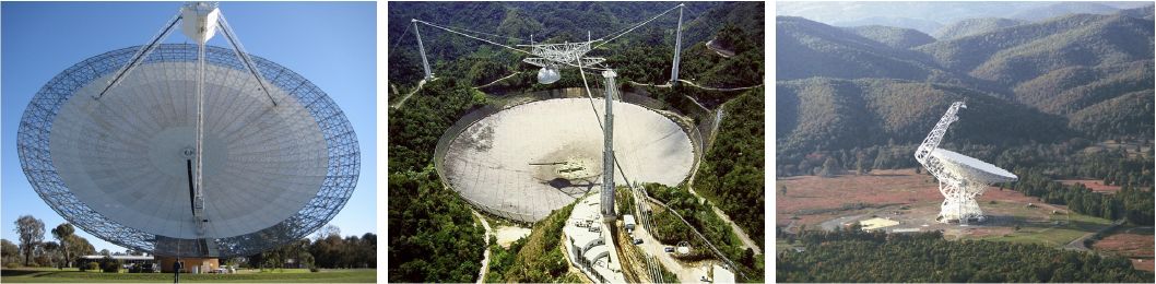 |
Figure 8. Examples of single-dish radio telescopes used to search for FRBs (from left to right): the 64-m Parkes telescope in New South Wales, Australia, the 305-m Arecibo telescope in Puerto Rico, USA, and the 110-m Green Bank Telescope in West Virgina, USA. |
The primary advantages of single dishes in FRB searches come from their large collecting areas (and thus high sensitivity) and low signal processing complexity. Their large focus cabins also have space for several wide bandwidth, cooled receivers, which are useful for studying FRB emission and polarization. Their sensitivity also makes them ideal instruments to follow up known FRBs to search for repetition, particularly in cases where the original detection was made with a less sensitive instrument (Connor and Petroff, 2018).
The greatest disadvantage of current single dishes is their poor localization of an FRB discovery: the localization uncertainty is θHPBW (often at least several arcminutes). Rejecting RFI in single-dish data can also be a challenge; however, this can be somewhat mitigated through multi-beam coincidence of candidates.
Even as we move into an era of interferometric FRB searches (Section 4.3.2), single dishes still have an important role to play in the study of FRB emission and polarization. Single dishes offer the raw sensitivity and broad frequency coverage (using a suite of receivers) to study FRB emission. For example, breakthroughs in the study of the repeating FRB 121102 (Section 5.4) have been made using receivers on single dishes at both higher and lower frequencies compared to the discovery observation. Future polarization studies of FRBs using sensitive single dishes are expected to provide further insights into the FRB emission mechanism (Section 8) and environment in their host galaxies. In the future, cooled phased array feeds (PAFs) installed on single dishes may result in better localization and increased survey speed (Deng et al., 2017).
4.3.2. Interferometric Methods
Interferometric radio telescopes are composed of many antennas or dishes, whose signals are combined to achieve, roughly speaking, the resolution of a single large telescope with a diameter equivalent to the longest baseline. The field of view can be sampled more finely using many beams, each created by applying different weightings or delays between different elements of the array. Radio interferometers come in a wide variety of shapes and sizes (Fig. 9). Some are made of smaller radio dishes such as the Jansky Very Large Array (JVLA, 27 25-m dishes), the Westerbork Synthesis Radio Telescope (WSRT, 14 25-m dishes), and the Australian Square Kilometre Array Pathfinder (ASKAP, 36 12-m dishes). Others consist of cylindrical parabaloids with many receivers sampling along the focal line, such as the Canadian Hydrogen Intensity Mapping Experiment (CHIME, 4 parallel 100-m long parabaloids) and the upgraded Molonglo Synthesis Telescope (UTMOST, 2 778-m long parabaloids). Others still are made from individual stationary dipole antennas such as the Low Frequency Array (LOFAR) and the Murchison Wide-field Array (MWA).
 |
Figure 9. Examples of radio interferometers used to search for FRBs (from left to right): the Jansky Very Large Array (JVLA) of 27 25-m dishes in New Mexico, USA, the Canadian Hydrogen Intensity Mapping Experiment (CHIME) with four cylindrical paraboloids each 100-m long and 20-m in diameter in British Columbia, Canada, and the core of the Low-Frequency Array (LOFAR) of dipoles in the Netherlands. |
FRB searches with interferometers can be done in a variety of ways (Colegate and Clarke, 2011). Incoherent searches discard phase information and use a summation of the individual element intensities; these have the advantage of large fields of view (equal to the primary field of view of the elements), but sensitivity scales as √N for N elements and localization precision is poor. Coherent searches create tied-array beams (TABs) by applying differential weights to different elements and summing the signals in phase; in this case sensitivity scales as N, thus providing both better sensitivity and better localization. However, beamforming with many elements can have high computational complexity requiring powerful backend hardware (Maan and van Leeuwen, 2017). Image plane FRB searches look for short transients through difference imaging, which takes advantage of existing imaging hardware on many interferometers; however, short duration images may be low sensitivity or poor quality making the identification of genuine astrophysical transients difficult. Additionally, image plane FRB data may have lower time resolution and thus miss fine-scale temporal structure in the bursts. However, if the imaging time is short (∼ms), it can still be possible to capture the basic information about the FRB such as DM and approximate pulse duration, as with the realfast system (Law et al., 2018).
General advantages to interferometric FRB searches are the flexible nature of interferometers in terms of pointing, localizing, and beam-forming, particularly if voltage data is recorded from each element upon detection of an FRB. The ability to track quickly, form sub-arrays, or do fly’s eye surveys to increase field of view make interferometers quite dynamic facilities (Shannon et al., 2018).
Interferometric FRB searches present substantial challenges. Combining data streams from many elements, coherently or incoherently, requires enormous computational power and large data rates. This becomes even more of a challenge when the goal is to search through incoming data for FRBs in real time. One dimensional arrays such as UTMOST and WSRT will also produce elongated beam shapes, making 2-D localization imprecise (though note that UTMOST is being upgraded to work as a 2-D array). Interferometers can also come with the penalty of reduced choice in observing band. Small dishes may lack the necessary space at the focus for multiple receivers at different frequencies, and dipole arrays may only be hardwired to operate at a specific set of frequencies. These may limit the information that can be gleaned from an individual FRB detection.
8 https://code.google.com/archive/p/dedisp/ and https://sourceforge.net/projects/heimdall-astro/ Back.
9 For example, prepsubband in presto, https://github.com/scottransom/presto Back.
10 See for example https://github.com/iansbrown/FRB-FDMT-Search/blob/master/FDMT_functions.py or a GPU implementation at https://github.com/ledatelescope/bifrost/blob/master/src/fdmt.cu Back.
11 https://github.com/cbassa/cdmt Back.
12 https://sourceforge.net/p/heimdall-astro/code/ci/master/tree/Pipeline/label_candidate_clusters.cu Back.
13 See also http://ascl.net/1807.014 for a machine learning-based approach Back.
14 https://sourceforge.net/p/heimdall-astro/code/ci/master/tree/Applications/coincidencer.C Back.
15 https://github.com/ckarako/rrattrap Back.
16 https://github.com/danielemichilli/SpS Back.
17 https://sourceforge.net/projects/heimdall-astro/ Back.
18 https://www.cv.nrao.edu/~sransom/presto/ Back.
19 https://github.com/AA-ALERT/AMBER Back.
20 https://github.com/kiyo-masui/burst_search Back.