


From the observed properties of the FRBs detected at various telescopes around the world, the next crucial but challenging step is to infer from observations the intrinsic physical properties of the population. Given that little is currently known about the progenitors and origins of FRBs this type of study is in its early stages. Nevertheless, efforts have already been made to extrapolate from the population of discovered FRBs to their population more globally. Here we summarize some results from FRB population studies and draw some conclusions from the publicly available sample of FRBs.
7.1. The fluence–dispersion measure plane
The current state of the FRB population as interpreted as a cosmological sample of sources is shown in Fig. 16. This sample includes the recent flurry of ASKAP discoveries and shows fluence versus inferred extragalactic DM for the Parkes and ASKAP samples as well as the repeater FRB 121102. The CHIME/FRB detections from CHIME/FRB Collaboration et al. (2019b) have not been plotted due to the uncertain flux calibration of the instrument, as emphasised in the discovery publication. From this diagram, we see evidence for a change of fluence with DM, which is expected for a population of sources at different distances. We note that the large scatter seen on this diagram is inconsistent with the idea of FRBs as standard candles. As can be seen from the overlaid curves, there is over an order of magnitude spread in the implied intrinsic luminosity. We also note that the distribution of pulse fluences for the repeater are dramatically different than the rest of the sample. Part of this difference could be due to a selection bias from the higher sensitivity of FRB 121102 observations that has come from observations with Arecibo. As underscored in the previous section, further follow-up observations of all FRBs with as high sensitivity as possible are required.
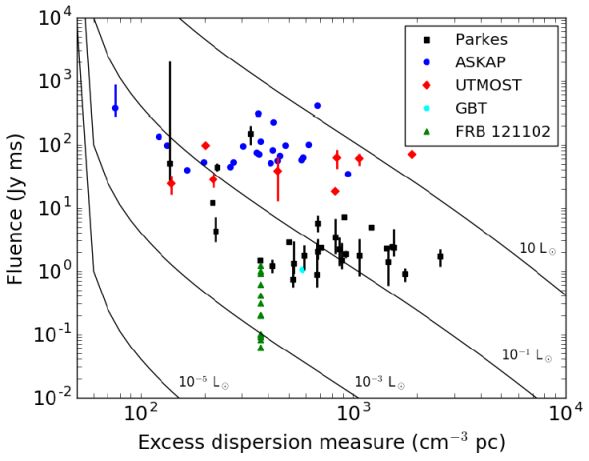 |
Figure 16. Fluence–dispersion measure distribution for the currently observed sample overlaid with lines of isotropic equivalent luminosity values assuming a contribution of DMHost = 50 cm−3 pc. The recent detections from CHIME/FRB have been omitted (see text). |
Although there are clearly a lot of selection biases inherent in shaping this diagram, the process of FRB detection is reasonably well understood. As a result, it is possible to set up a Monte Carlo simulation of the FRB population that can mimic the properties shown in Fig. 16 and allow us to infer the underlying, as opposed to the observed, distributions of population parameters. Population studies that attempt to account for these biases are now being used to help form a self-consistent picture on the FRB distribution and luminosity function. The Monte Carlo simulation process attempts to follow the process from emission of the signal to detection. A simulation typically proceeds by randomly drawing an FRB from intrinsic distributions of pulse widths and luminosities. Sources can be assigned distances based on an assumption about the underlying redshift distribution. Finally, assumptions about the electron content at the source, in the host galaxy, the IGM and the Milky Way can be made to infer the observed DM. With these ingredients, one can infer the observed pulse fluence and decide whether each model FRB is detectable or not.
A pioneering study of this kind, based on a sample of only 9 FRBs from Parkes known at the time, is described in Caleb et al. (2016a). A key result from this study was that, although the source distributions could be reproduced by a cosmological FRB population, the sample was not large enough to discriminate between spatial distributions that resulted from uniform density with co-moving volume, or whether they follow the well-known peak in star formation that occurs around z ∼ 1 (Madau and Dickinson, 2014). Similar results were also found with a slightly larger sample by Rane (2017). Both these studies estimate that sample sizes in the range 50–100 FRBs are needed to distinguish between different redshift distributions.
The overall form of the fluence–dispersion measure relationship in Fig. 16 can be understood in terms of a range of luminosities and host DMs that produces FRBs that are detectable out to different DM limits depending on telescope sensitivity. At the time of writing, the dominant contributions are ASKAP, which probes the bright low-DM part of the population, and Parkes, which is probing the fainter high-DM end. A recent population study by Lorimer (2018) suggests that this population will be extended to higher DMs in the future with the addition of sensitive FRB surveys with larger instruments. For example, FAST will more likely probe the FRB population with DMs above 2000 cm−3 pc (Zhang, 2018).
7.2. The FRB luminosity function
Although early analyses of the FRB population (e.g. Hassall et al., 2013, Lorimer et al., 2013) assumed, in the absence of further constraints, that the population of FRBs is consistent with them being standard candles, as mentioned above and as seen in Fig. 16, a distribution of luminosities is required to model the emerging samples of FRBs. This is perhaps unsurprising, given that FRBs may well have relatively narrow emission beams. While the shape of the luminosity function is currently not well understood, more recent analyses (see, e.g., Luo et al., 2018, Fialkov et al., 2018) seem to be favouring Schechter luminosity functions over power-law or normal distributions (Caleb et al., 2016a). The Schechter function gives the number of FRBs per unit logarithmic luminosity interval
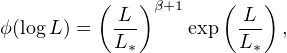 |
(24) |
where the power-law index β and cut-off luminosity L* are free parameters. This empirical characterization is motivated by success in modeling extragalactic luminosities in which very bright sources are rarer than expected from a straightforward power-law. Although, whether it will serve as an accurate characterization of the FRB luminosity function remains to be seen. Very recently, using a Bayesian-based Monte Carlo approach, Luo et al. (2018) prefer models with −1.8 < β < −1.2 and L* ∼ 5 × 10¹⁰ L⊙. Future progress in refining constraints on the form of this distribution, particularly at the low-luminosity end, could be made by detections of FRBs in nearby galaxy clusters (Fialkov et al., 2018). At the high-luminosity end, constraints on the emission mechanism may be possible from further studies of the fluence distribution (for further discussion, see Lu and Kumar, 2018b).
7.3. FRB rates and source counts
The estimated rate of observable FRBs is typically given as an all-sky
rate above some sensitivity limit rather than a volumetric or
cosmological rate, since the redshift distribution of FRBs is
unknown. Constraints on the all-sky rate
of FRBs,  , have been
carried out by a number of authors and are summarized in
Table 3.
, have been
carried out by a number of authors and are summarized in
Table 3.
| Rate | Range | CI |  lim lim |
Frequency | Reference |
| (FRBs sky−1 day−1) | (%) | (Jy ms) | (MHz) | ||
| ∼225 | — | — | 6.7 | 1400 | (Lorimer et al., 2007) |
| 10000 | 5000 – 16000 | 68 | 3.0 | 1400 | (Thornton et al., 2013) |
| 4400 | 1300 – 9600 | 99 | 4.4 | 1400 | (Rane et al., 2016) |
| 7000 | 4000 – 12000 | 95 | 1.5 | 1400 | (Champion et al., 2016) |
| 3300 | 1100 – 7000 | 99 | 3.8 | 1400 | (Crawford et al., 2016) |
| 587 | 272 – 924 | 95 | 6.0 | 1400 | (Lawrence et al., 2017) |
| 1700 | 800 – 3200 | 90 | 2.0 | 1400 | (Bhandari et al., 2018) |
| 37 | 29 – 45 | 68 | 37 | 1400 | (Shannon et al., 2018) |
All estimated rates are roughly consistent within the errors with
≳ 103 FRBs detectable over the whole sky every day
above a fluence threshold of ≳ 1 Jy ms. Under an assumption that these sources are
distributed cosmologically out to a redshift z ∼ 1 the
implied volumetric rates of roughly 2 × 10³
Gpc−3 yr−1 (of observable events)
are two orders of magnitude lower than the estimated core-collapse
supernova (CCSN) rate out to this redshift
(Dahlen
et al., 2004).
Rates of CCSN sub-classes vary considerably and the FRB rate may be consistent with Type Ib and Ic rates (Dahlen et al., 2012) but is still one to two orders of magnitude larger than the estimated rate of super-luminous supernovae (Prajs et al., 2017). While the all-sky GRB rate and the distribution of GRBs in redshift are highly uncertain, the observable FRB rate is still likely an order of magnitude larger than the total GRB rate in this redshift range, even when accounting for GRB events not beamed towards Earth (Frail et al., 2001). The binary neutron star merger rate is also highly uncertain but z = 0 estimates from the detections of the LIGO Virgo Collaboration (LVC) give a rate of RBNS = 1540−1220+3200 Gpc−3 yr−1 (Abbott et al., 2017b), broadly consistent with the merger rate as derived from Galactic BNS systems. Extrapolating these rates to larger distances with no cosmological evolution gives an event rate within an order of magnitude of the estimated FRB event rate, although perhaps slightly lower. If there is significant evolution in the rate of BNS mergers over redshift the true rate of merger events may be much lower when integrating to high redshift.
The high all-sky rate of FRB events relative to many other types of observable transients already places some constraints on their progenitors. Even for a cosmological distribution of events, if FRBs are generated in one-off cataclysmic events their sources must be relatively common and abundant. This becomes even more important for progenitors only distributed in the nearby volume, such as young neutron stars in supernova remnants (Connor et al., 2016b). However, if the high FRB rate is generated by a smaller population of repeating sources, the all-sky rate becomes slightly easier to account for and sources can be less common and far less numerous, but the engine responsible for repeating pulses must be relatively long-lived. Of the FRBs observed to-date, only two have been detected to repeat (see Section 5.4 and Section 5.5) and if all others repeat they are either infrequent, highly non-periodic, or may have very steep pulse-energy distributions.
Determinations of the FRB rate from survey observations are very useful
as they can be used to make predictions about other experiments without
the need for a lot of assumptions about the spatial distribution of the
population, or form of the luminosity function. The impact of the
underlying population can be encapsulated within the cumulative
distribution of event rate as a function of peak flux or, more
generally, fluence. This dependence is usually modeled as a power law
such that the rate above some fluence limit
min is given by
(>
min) ∝
minγ,
where the index γ = −1.5 for Euclidean geometry.
Since, for a survey with some instantaneous solid angle coverage Ω
with given amount of observing time T above some
min, the number
of detectable FRBs N(>
min) =
Ω T ∝
minγ this same index is often used to describe the
source count distribution.
In event rate or source count studies, there is currently a wide range of γ values that have been claimed so far beyond –1.5. Macquart and Ekers (2018) estimate, based on a recent maximum likelihood analysis on the Parkes FRBs, that γ = −2.6−1.3+0.7. In contrast, based on essentially the same sample of FRBs, Lawrence et al. (2017) estimate γ = −0.91 ± 0.34. Very recently, a combined analysis of the source counts for the ASKAP and Parkes samples by James et al. (2018) has found evidence for a break in the simple power-law dependence in which γ = −1.1 ± 0.2 for the fainter and more distant Parkes population and γ = −2.2 ± 0.5 for the brighter and more nearby ASKAP population. If confirmed by future studies, this would signify a cosmologically evolving FRB progenitor population peaking in the redshift range 1–3. This issue is likely to be investigated by further, more detailed Monte Carlo simulations and a larger available sample of FRBs.
One issue that has not been discussed extensively in the literature so far is to what extent the above FRB rates need to be scaled to account for beamed emission. This issue is well developed within the field of radio pulsars (see, e.g., Tauris and Manchester, 1998) where it is well known that this ‘beaming factor’ is of order 10 for canonical pulsars, i.e. we see only a tenth of the total population of active pulsars in the Galaxy. The rates shown in Table 3 are, therefore, for potentially observable FRBs only. When computing volumetric rates, it is important to consider this correction. Given the uncertain nature of FRBs at the present time this is highly speculative, but we urge theorists to specify as far as possible the likely beaming corrections in emission models.
As noted originally by Thornton et al. (2013), instrumental broadening of the pulses in systems that employ incoherent dedispersion can often account for a substantial fraction if not all of the observed pulse widths. In a recent study that carefully accounts for intrinsic and extrinsic contributions to FRB pulse profile morphology, Ravi (2019) demonstrates that, after accounting for pulse broadening due to scattering, only five of the sample of seventeen Parkes FRBs he analyzed have widths that exceed that predicted by dispersion broadening. Six FRBs in this sample are temporally unresolved. While a larger sample of FRBs in future will definitely help, it is true that current instrumentation cannot resolve a significant number of currently detectable FRB pulses.
The difficulties in observing FRBs over large bandwidths have so far hampered attempts to quantify their broadband spectra. As mentioned in Section 2.1, the simplest model is to adopt a power-law dependence with flux density S ∝ να for some spectral index α. Many statistical analyses either remain agnostic about the spectrum and posit ‘flat spectra’, i.e. α = 0, or assume (without strong justification) that FRBs have a spectral dependence similar to that observed for pulsars, where α ∼ −1.4 (Bates et al., 2013).
The most stringent constraints on α come from non-detections of FRBs at radio frequencies below 400 MHz. Chawla et al. (2017) use the lack of FRB detections in the Green Bank Northern Celestial Cap survey to limit α > −0.9. Similarly, the lack of FRBs found with LOFAR limit α > +0.1 (Karastergiou et al., 2015). These constraint from lower frequencies are strongly at odds with a recent study of the ASKAP FRBs (Macquart et al., 2018) which finds α = −1.6−0.2+0.3, i.e. similar to the normal pulsar spectra.
These disparate results imply that the spectral behaviour of FRBs likely involves a turnover at sub-GHz frequencies or may not follow a power-law at all but in fact be in emission envelopes (e.g., Hessels et al., 2018, Gourdji et al., 2019). It is important to note that scattering may also play a significant role at low frequncies, artificially shallowing the measured spectral index of FRBs. CHIME/FRB Collaboration et al. (2019b) show that a large fraction of their sample at low frequencies exhibits significant scattering.
Spectral behaviour with a turnover might be observed in future for FRBs embedded in dense ionized media. As pointed out by Kulkarni et al. (2014) and Rajwade and Lorimer (2017), and is known to be exhibited in some radio pulsars, free-free absorption from a shell surrounding an FRB can result in substantial modifications to the spectra, which might result in turnovers at decametric wavelengths. Very recently, in a comprehensive review of other propagation effects on FRB spectra, Ravi and Loeb (2018) show that spectral turnovers might be ubiquitous, regardless of the emission mechanism. Future surveys at these wavelengths might also observe the effect of spectral turnovers occurring at higher frequencies that are being redshifted into the < 500 MHz band (Rajwade and Lorimer, 2017).