


Following an introduction to the observed properties of FRBs, we discuss some basic physical inferences that can be made from the most readily observable parameters. A selection of the current sample of FRBs is shown in Fig. 3, which displays all those found with the Parkes telescope to date.
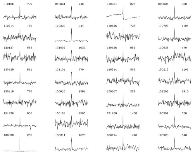 |
Figure 3. Compilation showing the first twenty-eight FRBs discovered using the Parkes telescope. The detections are arranged in order of date. Each light curve shows a 2-s window around the pulse. Following gamma-ray burst notation, the FRBs are named in YYMMDD format to indicate the year (YY) month (MM) and day (DD) on which the burst was detected. Also listed to the right of each pulse are the observed dispersion measures (DMs) in units of cm−3 pc. |
The FRB search process is described in detail in Section 4. In brief, it consists of looking for dispersed pulses like the one shown in Fig. 1 in radio astronomical data that is sampled in frequency and time. Searches are most commonly done by forming a large number of time series corresponding to different amounts of dispersion over a wide range. The amount of dispersion is quantified by the time delay of the pulse between the highest and lowest radio frequencies of the observation, νhi and νlo are the high, respectively, as
 |
(1) |
where me is the mass of the electron, and c is the speed of light. The second approximate equality holds when νlo and νhi are in units of GHz. The dispersion measure is given as
 |
(2) |
In this expression, ne is the electron number density, l is a path length and d is the distance to the FRB, which we will estimate below. Note that, as in pulsar astronomy, DM is typically quoted in units of cm−3 pc. This makes the numerical value of DM more easy to quote compared to using column density units of, e.g., cm−2. In practice, depending on the observational setup and signal-to-noise ratio (S/N), the DM can be measured with a precision of about 0.1 cm−3 pc.
The process for finding the optimum DM of a pulse is described in Section 4.1. Once the DM value has been optimised, a de-dispersed time series can be formed in which the pulse S/N is maximized. If this time series can be calibrated such that intensity can be converted to flux density as a function of time, S(t), the pulse can be characterized in terms of its width and peak flux density, Speak. In practice, the calibration process is approximated from a measurement of the root-mean-square (rms) fluctuations in the dedispersed time series, σS. From radiometer noise considerations (see, e.g., Lorimer and Kramer, 2012),
 |
(3) |
where Tsys is the system temperature, G is the antenna gain, Δν is the receiver bandwidth and tsamp is the data sampling interval.
For each FRB, the observed pulse width, W, is typically thought of as a combination of an intrinsic pulse of width Wint and instrumental broadening contributions. In general, for a top-hat pulse,
 |
(4) |
where tsamp is the sampling time as above, ΔtDM is the dispersive delay across an individual frequency channel and ΔtDMerr represents the dispersive delay due to de-dispersion at a slightly incorrect DM. FRB pulses can also be temporally broadened by multi-path propagation through a turbulent medium. The so called ‘scattering time-scale’ τs due to this effect is discussed in detail in Section 3.3.
Pulse width is often measured at 50% and 10% of the peak (Lorimer and Kramer, 2012); however, for a pulse of arbitrary shape, it is also common to quote the equivalent width Weq of a top-hat pulse with the same Speak. Such a pulse has an energy or fluence
 |
(5) |
A complicating factor with quoting flux density or fluence values is the fact that, for many FRBs, the true sky position is not known well enough to uniquely pinpoint the source to a position in the beam. Here, ‘beam’ is defined as the field of view of the radio telescope, which is typically diffraction limited, as discussed more in Section 4.3.1. The sensitivity across this beam is not uniform, with the response as a function of angular distance from the center being approximately Gaussian, in most cases. As a result, with the exception of the ASKAP FRBs (Bannister et al., 2017, Shannon et al., 2018) most one-off FRB fluxes and fluences determined so far are lower limits. In addition, the limited angular resolution of most FRB searches so far leads to typical positional uncertainties that are on the order of a few arcminutes.
As is commonly done for other radio sources, measurements of the flux density spectrum of FRBs as described by Sν ∝ να, where α is the spectral index, are typically complicated by the small available observing bandwidth. As a result, α is usually rather poorly constrained. An additional complication also arises from the poor localization of FRBs within the telescope beam, where the uncertain positional offset and variable beam response with radio frequency can lead to significant variations in measured α values. We also note that a simple power-law spectral model may not be an optimal model of the intrinsic FRB emission process (e.g., Hessels et al., 2018). As discussed in Section 3, the spectrum can also be modified by propagation effects.
One exception to these positional uncertainty limitations is the repeating source FRB 121102, which is discussed further below (Section 5.4). We note here that flux density S(t) defined above is the integral of the flux per unit frequency interval over some observing band from νlo to νhi. For the purposes of the discussion below, and in the absence of any spectral information, we assume α = 0 so that
 |
(6) |
For a few FRBs, measurements of polarized flux are also available (see, e.g., Petroff et al., 2015a, Masui et al., 2015, Ravi et al., 2016, Michilli et al., 2018a). In these cases it is often possible to measure the change in the position angle of linear polarization, which scales with wavelength squared. As discussed in Section 3.4, the constant of proportionality for this scaling is the rotation measure (RM), which probes the magnetic field component along the line of sight, weighted by electron density.
For most FRBs, the only observables are position, flux density, pulse width, and DM. We now provide the simplest set of derived expressions that can be used to estimate relevant physical parameters for FRBs.
Starting with the observed DM, we follow what is now tending towards standard practice (see, e.g., Deng and Zhang, 2014) and define the dispersion measure excess
 |
(7) |
where DMMW is the Galactic (i.e. Milky Way) contribution from this line of sight, typically obtained from electron density models such as NE2001 (Cordes and Lazio, 2002) or YMW16 (Yao et al., 2017), DMIGM is the contribution from the intergalactic medium (IGM) and DMHost is the contribution from the host galaxy. The (1 + z) factor accounts for cosmological time dilation for a source at redshift z. The last term on the right-hand side of Eq. 7 could be further broken down into host galaxy free electrons and local source terms, as needed. In any case, DMe provides an upper limit for DMIGM, and most conservatively DMIGM < DMe. We note that DMMW is likely uncertain at least at the tens of percent level, but could in rare cases be quite far off if there are unmodelled Hii regions along the line of sight (Bannister and Madsen, 2014).
To find a relationship between DM and z, following, e.g., Deng and Zhang (2014), one can assume all baryons are homogeneously distributed and ionized with an ionization fraction x(z). In this case, the mean contribution from the IGM,
 |
(8) |
where the constant KIGM = 933 cm−3 pc assumes standard Planck cosmological parameters 3 and a baryonic mass fraction of 83% (Yang and Zhang, 2016) and Ωm and ΩΛ are, respectively, the energy densities of matter and dark energy. At low redshifts, the ionization fraction x(z) ≃ 7/8, and we find (see Fig. 1a of Yang and Zhang, 2016) DMIGM ≃ z 1000 cm−3 pc. For a given FRB with a particular observed DM, a very crude but commonly used rule of thumb is to estimate redshift as z < DM / 1000 cm−3 pc.
Finally, to convert this redshift estimate to a luminosity distance, dL, we can make use of the approximation 4 dL ≃ 2z(z + 2.4) Gpc, which is valid for z < 1. In this case, for the most conservative assumption, we find that
 |
(9) |
For the repeating FRB 121102, where dL can be inferred directly from the measured redshift of the host galaxy, and constraints on dispersion in the host galaxy can be made, these expressions can be used instead to place constraints on DMIGM, as discussed in Section 5.4.
Having obtained a distance limit, for an FRB observed over some bandwidth Δν, we can place constraints on the isotropic equivalent source luminosity
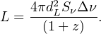 |
(10) |
In arriving at this expression, we have started from the differential flux
per unit logarithmic frequency interval,
Sν Δ ν (see, e.g. Eq. 24 of
Hogg,
1999)
in the simplest case of a flat spectrum source (i.e. constant
Sν, see Eq. 6). The (1 + z) factor accounts
for the redshifting of the frequencies between
the source and observer frames. We also note that replacing
Sν with
fluence  in the above
expression yields the equivalent isotropic
energy release for a flat spectrum source.
in the above
expression yields the equivalent isotropic
energy release for a flat spectrum source.
As an example, we apply Eq. 9 to a typical FRB (FRB 140514) with a DM of 563 cm−3 pc and a peak flux density of 0.5 Jy. The limiting luminosity distance dL < 3.3 Gpc, i.e. z < 0.56. The limiting luminosity L < 44 Jy Gpc2 per unit bandwidth. Assuming a 300-MHz bandwidth, this translates to a luminosity release of approximately 1017 W (1024 erg s−1).
As shown by Yang et al. (2017), for z < 1, the luminosity distance can be directly related to the IGM DM as follows:
 |
(11) |
Yang et al. (2017) find the following useful approximate relationship:
 |
(12) |
where the constant K can be computed in terms of the assumed values of the constants in Eq. 11 at a particular observing frequency (for details, see Yang et al., 2017). Such a trend is apparent in the observed sample, albeit with a considerable amount of scatter. Applying this model to the FRBs found with the Parkes telescope, the authors constrain host galaxy DMs to have a broad distribution with a mean value ⟨ DMHost ⟩ = 270−110+170 cm−3 pc and L ∼ 1036 W (∼ 1043 erg s−1).
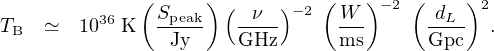
As in the case of other radio sources, where the emission mechanism is likely to be non-thermal in origin, it is often useful to quote the brightness temperature inferred from the source, TB, which is defined as the thermodynamic temperature of a black body of equivalent luminosity. Making similar arguments as is commonly done for pulsars (see, e.g., Section 3.4 of Lorimer and Kramer, 2012), we find
 |
(13) |
Again evaluating this for our example FRB 140514 from the previous section, where the pulse width W = 2.8 ms, we find TB < 3.5 × 1035 K.
3 For details, see Eq. 6 of Yang & Zhang (2016). Back.
4 This result is not widely used, but can be easily verified by numerical integration. Back.