2. DATA

2.1. ⁴He

The primordial ⁴He abundance is best determined from observations of HeII -> HeI recombination lines in extragalactic HII (ionized hydrogen) regions. There is a good collection of abundance information on the ⁴He mass fraction, Y, O/H, and N/H in over 70 such regions [8, 9, 10]. Since ⁴He is produced in stars along with heavier elements such as Oxygen, it is then expected that the primordial abundance of ⁴He can be determined from the intercept of the correlation between Y and O/H, namely Y_P = Y(O/H -> 0). A detailed analysis [11] of the data found

(1)

The first uncertainty is purely statistical and the second uncertainty is an estimate of the systematic uncertainty in the primordial abundance determination. The solid box for ⁴He in Figure 1 represents the range (at 2_stat) from (1). The dashed box extends this by including the systematic uncertainty. The He data is shown in Figure 2.

Figure 2. The Helium (Y) and Oxygen (O/H) abundances in extragalactic HII regions, from refs. [8] and from ref. [10]. Lines connect the same regions observed by different groups. The regression shown leads to the primordial 4He abundance given in Eq. (1).

The helium abundance used to derive (1) was determined using assumed electron densities n in the HII regions obtained from SII data. Izotov, Thuan, & Lipovetsky [9] proposed a method based on several He emission lines to ``self-consistently'' determine the electron density. Their data using this method yields a higher primordial value

(2)

As one can see, the resulting primordial ⁴He abundance shows significant sensitivity to the method of abundance determination, leading one to conclude that the systematic uncertainty (which is already dominant) may be underestimated. Indeed, the determination (1) of the primordial abundance above is based on a combination of the data in refs. [8], which alone yield Y_P = 0.228 ± 0.005, and the data of ref. [10] (based on SII densities) which give 0.239 ± 0.002. The abundance (2) is based solely on the self-consistent method yields and the data of [10]. One should also note that a recent determination [12] of the ⁴He abundance in a single object (the SMC) also using the self consistent method gives a primordial abundance of 0.234 ± 0.003 (actually, they observe Y = 0.240 ± 0.002 at [O/H] = -0.8, where [O/H] refers to the log of the Oxygen abundance relative to the solar value, in the units used in Figure 2, this corresponds to 10⁶O/H = 135). Therefore, it will useful to discuss some of the key sources of the uncertainties in the He abundance determinations and prospects for improvement. To this end, I will briefly discuss, the importance of reddening and underlying absorption in the H line line measurements, Monte Carlo methods for both H and He, and underlying absorption in He.

The He abundance is typically quoted relative to H, e.g., He line strengths are measured relative to . The H data must first be corrected for underlying absorption and reddening. Beginning with an observed line flux F(, and an equivalent width W(), we can parameterize the correction for underlying stellar absorption as

(3)

The parameter a is expected to be relatively insensitive to wavelength. A reddening correction is applied to determine the intrinsic line intensity I() relative to

(4)

where f() represents an assumed universal reddening law and C(H) is the correction factor to be determined. By minimizing the differences between X_R() to theoretical values, X_T(), for = H H and H, one can determine the parameters a and C(H) self consistently [13], and run a Monte Carlo over the input data to test the robustness of the solution and to determine the systematic uncertainty associated with these corrections.

In Figure 3 [13], the result of such a Monte-Carlo based on synthetic data with an assumed correction of 2 Å for underlying absorption and a value for C(H) = 0.1 is shown. The synthetic data were assumed to have an intrinsic 2% uncertainty. While the mean value of the Monte-Carlo results very accurately reproduces the input parameters, the spread in the values for a and C(H) are considerably larger than one would have derived from the direct ² minimization solution due to the covariance in a and C(H).

Figure 3. A Monte Carlo determination of the underlying absorption a (in Å ), and reddening parameter C(H), based on synthetic data.

Next one can perform an analogous procedure to that described above to determine the ⁴He abundance [13]. We again start with a set of observed quantities: line intensities I() which include the reddening correction previously determined along with its associated uncertainty which includes the uncertainties in C(H); the equivalent width W(); and temperature t. The Helium line intensities are scaled to H and the singly ionized helium abundance is given by

(6)

where E() / E(H) is the theoretical emissivity scaled to H. The expression (6) also contains a correction factor for underlying stellar absorption, parameterized now by a_HeI, a density dependent collisional correction factor, (1 + )^-1, and a flourecence correction which depends on the optical depth . Thus y⁺ implicitly depends on 3 unknowns, the electron density, n, a_HeI, and .

One can use 3-6 lines to determine the weighted average helium abundance, . From , we can calculate the ² deviation from the average, and minimize ², to determine n, a_HeI, and . Uncertainties in the output parameters are also determined. In principle, under the assumption of small values for the optical depth (3889), it is possible to use only the three bright lines 4471, 5876, and 6678 and still solve self-consistently for He/H, density, and a_HeI. Of course, because these lines have relatively low sensitivities to collisional enhancement, the derived uncertainties in density will be large.

The addition of 7065 was proposed [9] as a density diagnostic and then, 3889 was later added to estimate the radiative transfer effects (since these are important for 7065). Thus the five line method has the potential of self-consistently determining the density and optical depth in the addition to the ⁴He abundance. The procedure described here differs somewhat from that proposed in [9], in that the ² above is based on a straight weighted average, where as in [9] the difference of a ratio of He abundances (to one wavelength, say 4471) to the theoretical ratio is minimized. When the reference line is particularly sensitive to a systematic effect such as underlying stellar absorption, this uncertainty propagates to all lines this way.

Adding 4026 as a diagnostic line increases the leverage on detecting underlying stellar absorption. This is because the 4026 line is a relatively weak line. However, this also requires that the input spectrum is a very high quality one. 4026 is also provides exceptional leverage to underlying stellar absorption because it is a singlet line and therefore has very low sensitivity to collisional enhancement (i.e., n) and optical depth (i.e., (3889)) effects.

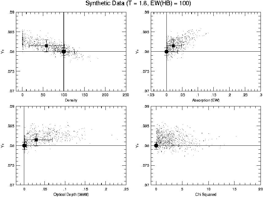
Figure 4. Results of modeling of 6 synthetic He I line observations. The four panels show the results of a density = 100 cm-3, aHeI = 0, and (3889) = 0 model.

As in the case of the hydrogen lines, Monte-Carlo simulation of the He data can be used to test the robustness of the solution for n, a_HeI, and [13]. Figure 4 presents the results of modeling of 6 synthetic He I line observations. The four panels show the results of a density = 100 cm^-3, a_HeI = 0, and (3889) = 0 model. The solid lines show the input values (e.g., He/H = 0.080) for the original calculated spectrum. The solid circles (with error bars) show the results of the ² minimization solution (with calculated errors) for the original synthetic input spectrum. The small points show the results of Monte Carlo realizations of the original input spectrum. The solid squares (with error bars) show the means and dispersions of the output values for the ² minimization solutions of the Monte Carlo realizations.

Figure 4 demonstrates several important points. First, the ² minimization solution finds the correct input parameters with errors in He/H of about 1% (less than the 2% errors assumed on the input data, showing the power of using multiple lines). There is a systematic trend for the Monte Carlo realizations to tend toward higher values of He/H. This is because, the inclusion of errors has allowed minimizations which find lower values of the density and non-zero values of underlying absorption and optical depth. Note that the size of the error bars in He/H have expanded by roughly 50% as a result. We can conclude from this that simply adding additional lines or physical parameters in the minimization does not necessarily lead to the correct results. In order to use the minimization routines effectively, one must understand the role of the interdependencies of the individual lines on the different physical parameters. Here we have shown that trade-offs in underlying absorption and optical depth allow for good solutions at densities which are too low and resulting in helium abundance determinations which are too high. Note that in the lower right panel of Figure 4 that the values of the ² do not correlate with the values of y⁺. The solutions at higher values of absorption and y⁺ are equally valid as those at lower absorption and y⁺.

Figure 5. Similar plot to Figure 4 except that the underlying absorption is 0.1 Å and (3889) = 0.1.

Figure 5 shows the results of the Monte Carlo when both and a_HeI 0, and n = 100 cm^-3. It is encouraging that in perhaps more realistic cases where the input parameters are non-zero, we are able to derive results very close to their correct values. The average of Monte Carlo realizations is remarkably close to the straight minimization for all of the derived parameters (n, a_HeI, and y⁺). However, there is an enormous dispersion in these results due to the degeneracy in the solutions with respect to the physical input parameters. This results in error estimates for parameters which are significantly larger than in the straight minimization. For example, the uncertainties in both the density and optical depth are almost a factor of 3 times larger in the Monte Carlo. When propagated into the uncertainty in the derived value for the He abundance, we find that the uncertainty in the Monte Carlo result (which we argue is a better, not merely more conservative, value) is a factor of 2.5 times the uncertainty obtained from a straight minimization using 6 line He lines. This amounts to an approximately 4% uncertainty in the He abundance, despite the fact that we assumed (in the synthetic data) 2% uncertainties in the input line strengths. This is an unavoidable consequence of the method - the Monte Carlo routine explores the degeneracies of the solutions and reveals the larger errors that should be associated with the solutions.

In Figure 6, I show the result of a single case based on the data of ref. [10] for SBS1159+545. Here, the helium abundance and density solutions are displayed. The vertical and horizontal lines show the position of the solution in [10]. The circle shows the position of the our solution to the minimization, and the square shows the position of the mean of the Monte-Carlo distribution. The spread shown here is significantly greater than the uncertainty quoted in [10].

Figure 6. A Monte Carlo determination of the helium abundance and electron density (in cm-3) for the region SBS11159+545. Solutions for a' and are not shown here.