Annu. Rev. Astron. Astrophys. 1988. 26: 631-86 Copyright © 1988 by Annual Reviews. All rights reserved

3. THE CLUSTER CORRELATION FUNCTION

3.1. Introduction

The spatial distribution of rich clusters of galaxies and the clustering properties of clusters have been the subject of considerable interest over the past two decades, with a wide range of claims as to the nature and properties of such clustering. Since rich clusters can be used rather efficiently in surveying the structure in large volumes of space, they have recently become an important tool in tracing the large-scale structure of the Universe.

The Abell (1958) catalog of rich clusters has been analyzed by many investigators (e.g. Abell 1958, 1961, Hauser & Peebles 1973, Rood 1976, Bahcall & Soneira 1983, 1984, Klypin & Kopylov 1983, Bahcall et al. 1986, Shvartsman 1988, Kalinkov et al. 1985, Batuski & Burns 1985a, Tully 1986, and references therein) using different techniques in an attempt to determine the spatial distributions of rich clusters. Abell (1958, 1961) found that the surface distribution of the clusters in his statistical sample (see Section 2) was highly nonrandom and reported evidence suggestiug the existence of superclusters; Bogart & Wagoner (1973), Hauser & Peebles (1973), and Rood (1976) (see also references therein) also found, using nearest-neighbor distributions and/or angular correlation functions, strong evidence for superclustering among the Abell clusters. The studies dealt primarily with the surface distribution of clusters and, in some cases, used approximate estimates for cluster redshifts. More recently, Bahcall & Soneira (1983, 1984) and, independently, Klypin & Kopylov (1983) used redshift measurements of complete samples of clusters to determine directly the spatial distribution of rich clusters. The results, discussed in more detail below, indicate that rich clusters of galaxies cluster very strongly in space, forming clusters of clusters of galaxies, or superclusters (see also Section 6). The clustering strength of clusters was observed to be much higher than the clustering strength of galaxies. The clustering or correlation scale for rich clusters was found to be about five times larger than the correlation scale of galaxies. Similar investigations followed therefore after (see below), all yielding consistent results. Since these results provide strong constraints on models for the formation and evolution of galaxies and structure, I review in this section the findings of recent investigations of the clustering of clusters, using various catalogs and methods.

The correlation function (Limber 1953, Peebles 1980a) is one of the best statistical tools to measure quantitatively the clustering of objects in a sample, yielding both clustering strength and extent. The joint probability dP() of finding two objects in a sample separated by an angle and within solid angles d₁ and d₂ is written as

(1)

where w() is the two-point angular correlation function and N is the surface number density of objects in the sample. The two-point angular correlation function thus describes, as a function of angular scale, the net projected pair clustering of objects on the sky above that expected from random distribution.

Similarly, the spatial correlation function (r) is defined by the joint probability dP(r) of finding two objects separated by a distance r and within volume elements dV₁ and dV₂, such that

(2)

where n is the space density of objects in the sample. The correlations are therefore zero for a random distribution of points and are positive for a clumped distribution on the relevant clumping scale.

3.2. Cluster Correlations

3.2.1   ABELL CLUSTERS   The two-point spatial correlation function of clusters, _cc(r), was determined by Bahcall & Soneira (1983; hereinafter BS83) using Abell's (1958) statistical sample of rich clusters of galaxies of distance class D 4 (z 0.1), with redshifts for all clusters reported by Hoessel et al. (1980). (For properties of the Abell catalog, see Section 2.) This sample includes all 104 Abell clusters at D 4 that are of richness class R 1 and are located at high Galactic latitude (|b| 30°). A summary of the sample properties and its division into distance and richness classes, as well as into hemispheres, is presented in Table 1 and BS83. Also listed in Table 1 and BS83 are properties of the much larger and deeper D = 5 + 6 statistical sample (z 0.2) that includes 1547 clusters. While only a small fraction of the redshifts are measured for this sample, it was used, because of its much larger number of clusters, in various comparison tests to strengthen and confirm the results obtained from the D 4 sample.

The frequency distribution F(r) for all pairs of clusters with separation r in the sample was determined. In order to minimize the influence of selection effects on the determination of (r), a set of 1000 random catalogs was constructed, each containing 104 clusters randomly distributed within the angular boundaries of the survey region but with the same selection functions in both redshift, n(z), and latitude, P(b), as the Abell redshift sample. The frequency distribution of cluster pairs was determined in both the real and random catalogs, and the results were then compared. This procedure ensures that the selection effects and boundary conditions will affect the data and random catalogs in the same manner.

The spatial correlation function was determined from the relation

(3)

where F(r) is the observed frequency of pairs in the Abell sample, and F^R(r) is the corresponding frequency of random pairs (as determined by the ensemble average frequency of the 1000 random catalogs). An ensemble average random frequency is used in order that (r) not be affected by the fluctuations present in any particular realization of a single random sample. The correlation function was evaluated for various cases, including (a) no selection function in latitude [i.e. P(b) = 1]; (b) full selection function in latitude; (c) Northern and Southern Hemispheres treated separately; and (d) high- and low-latitude zones (|b| > 50° and |b| 50°) treated separately, each with its observed n(z) [and P(b)] selection function.

The resulting correlation function is presented in Figure 3. Strong spatial correlations are observed at separations 25h^-1 Mpc. Weaker correlations are observed to larger separations of at least ~ 50h^-1 Mpc, and possibly ~ 100h^-1 Mpc, where _cc ~ 0.1; beyond 150 h^-1 Mpc, no statistically significant correlations are observed in the present sample.

The correlation function of Figure 3 can be well approximated by a single power-law relation of the form _cc(r) = 300 r^-1.8 for 5 r 150h^-1 Mpc. The function is smooth, with little scatter at r 50h^-1 Mpc. At r > 50h^-1 Mpc, the scatter and uncertainties increase, but weak correlations of order 0.2 are still detected at these very large separations. When corrected for velocity broadening among clusters, the intrinsic rich (R 1) cluster correlation function was determined by Bahcall & Soneira to be (BS83)

Figure 3. (Top) The spatial correlation function of the D 4 Abell cluster sample (BS83). [Crosses refer to no correction for latitude selection function; dots refer to the full correction of P(b).] The solid line is the best-fit -1.8 power law to the data. The dashed line is the galaxy-galaxy correlation function of Groth & Peebles (1977). (Bottom) Same as (top) but plotted in larger bins at large separations.

(4)

In comparison, the correlation function of galaxies is given by (Groth & Peebles 1977, Davis & Peebles 1983)

(5)

The rich cluster correlation function has the same shape and slope as those of the galaxy correlation function, but it is considerably stronger at any given scale (by a factor of ~ 18) than the correlation function of galaxies. The cluster correlations also extend to greater separations than the scales observed in the galaxy correlations. The cluster correlation scale length, i.e. the scale at which the correlation function is unity, is r₀ 26h^-1 Mpc (Equation 4), as compared with r₀ 5h^-1 Mpc for galaxies. The extent of the rich cluster correlation function beyond the reported ~ 15h^-1 Mpc break in the galaxy correlation function (Groth & Peebles 1977) suggests the existence of large-scale structure in the Universe (~ 15h^-1 Mpc). While the reason for the strong increase of correlation strength and scale from galaxies to clusters is still a theoretical challenge, some possible explanations are discussed in Sections 5 and 9. The cluster correlation function determined above places constraints on models for the formation of galaxies and structure (see Section 9).

In order to ensure that the spatial correlation function is not due to some special peculiarities in the nearby D 4 sample. Bahcall & Soneira (BS83) carried out several tests that are discussed below.

First, the angular correlation function of the much larger and deeper D = 5 + 6 sample (1547 R 1 clusters to z 0.2) was determined and compared with that expected from the spatial correlation function above (Equation 4), as well as from the expected scaling law (Peebles 1980a) of the D 4 angular correlation function. The angular correlation functions of the nearby D 4 and distant D = 5 + 6 samples are determined to be (BS83)

	(6)
	(7)

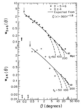
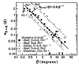
The angular correlations scale as expected from the scaling law applied to their respective distances. A comparison of the scaled functions is shown in figure 4. If the correlations were mainly due to patchy obscuration or other omissions by Abell, the (observed) scaling would not be expected. The scaling agreement indicates that any possible projection biases in the catalog (e.g. Sutherland 1988) are rather small and do not significantly affect the correlation results (see Bahcall 1988b, Dekel 1988). The reduced correlation scale suggested by Sutherland may result from overcorrecting the actual correlation power on large scales. A comparison of the D = 5 + 6 angular function with that expected from the spatial correlation function of Equation (4), when integrated over the relevant redshift distribution, is shown in Figure 5. The agreement between the D 4 and D = 5 + 6 functions is excellent. This agreement indicates that the D 4 redshift sample is a fair sample of the much larger sample, and that the observed correlations represent real correlations of clusters in space. The scaling law of the angular functions was also studied by Hauser & Peebles (1973), who reached similar conclusions with regard to the reality of the intrinsic correlations.

Figure 4. (a) The angular correlation function of the D 4 Abell cluster sample (BS83). (b) The angular correlation function of the deep D = 5 + 6 sample (squares). Open circles are the angular correlation function of the D 4 sample (Figure 4a) scaled by the standard scaling law of an intrinsic spatial correlation using the distance ratio of the two samples (Section 3). (Correlations of 0.05 are rather uncertain.) The position of the mean Abell radius is indicated by the arrow.

Third, the angular correlation function of the D = 5 + 6 sample was determined in different regions of the sky, yielding consistent results within the uncertainties (see Figure 6).

These tests, and those listed in Section 3.3 below, suggest that the observed cluster correlation function is mostly due to physical clustering of rich clusters of galaxies that extends to large scales.

Figure 5. The curves represent the angular correlation function expected from an intrinsic cluster spatial function given by (r) = 360r-1.8 for r rc (Equation 4), and the sample selection function with redshift n(z) (BS83). The top represents the expectation for the D = 5 + 6 Abell sample, and the bottom, the expectation for the D 4 sample. Different cutoffs rc of the intrinsic spatial function are marked. The expected curves are compared with the observed angular correlation functions of the D = 5 + 6 (dots) and D 4 (circles) samples. The position of the mean Abell radius, below which no pairs exist, is marked by the arrow for each sample (Section 3.2).

Since the correlation strength appears to increase from galaxies to clusters, Bahcall & Soneira also investigated whether a similar trend is observed between the correlation function of poor and rich clusters. The angular correlation functions of different richness classes (R = 1 and R 2) were determined for the large D = 5 + 6 sample (1125 R = 1 clusters, 422 R 2 clusters). The amplitude of the correlation function was found to be strongly dependent on cluster richness, with richer clusters (R 2) showing stronger correlations by a factor of ~ 3 as compared with the poorer (R = 1) clusters. The results are shown in Figure 7. Both richness classes exhibit the same power-law shape correlation function as observed in the total sample; they satisfy

(8)

Figure 6. The angular correlation function of the D = 5 + 6 Abell cluster sample for different zones: Northern Hemisphere (squares); Southern Hemisphere (circles); high latitude, |bII| 50° (crosses); and the total sample (dots). (A very strong south-polar apparent super-cluster increases somewhat the southern correlations at small separations.) Other zones of low latitude (|bII| = 30 - 50°) and different longitudes yield similar results (BS83).

Figure 7. The angular correlation function of richness 1 and richness 2 Abell clusters in the D = 5 + 6 sample (BS83).

(9)

The implied spatial correlation can then be represented by

	(10)
	(11)

The amplitude of the total (R 1) correlation function is dominated by the lower amplitude of the poorer, but more numerous, R = 1 clusters. Figure 8 shows the dependence of the correlation function on the richness of the system, from single galaxies to poor and rich clusters, as suggested by BS83 (see also Section 3.5 for a more updated richness dependence). The correlations become stronger with increasing richness (or luminosity) of the system, suggesting that the correlation function depends upon richness. The galaxy-cluster cross-correlation function (Seldner & Peebles 1977; see, however, Efstathiou 1988 (also Section 3.2.4)] is consistent with the cluster correlations and the trend observed above (Figure 8). Recent observations of clusters of different types and richnesses (see summary below) yield results that are consistent with the richness trend suggested by BS83 (Section 3.5).

Figure 8. The dependence on richness of the two-point spatial correlation function suggested by BS83. The spatial correlation function at r = 5h-1 Mpc is plotted as a function of richness for the galaxy-galaxy, galaxy-cluster, and cluster-cluster pairs (R 1, as well as R = 1 and R 2 independently; the latter two are shown by open circles). The dashed line, (n) n0.8, is presented in order to guide the eye in the approximate richness dependence of the correlation (Sections 3.2, 3.5).

Klypin & Kopylov (1983) investigated the spatial correlation function of a nearby sample of Abell clusters similar to the one described above, supplementing available redshift data with their own observations. Their sample includes 158 Abell clusters of all richness classes [R 0 (i.e. including the somewhat incomplete class of R = 0 clusters] in distance group D 4 and located at |b| 30°. Their results are consistent with those of BS83. They find _cc(r) = (r/25)^-1.6 for their observed range of r 50h^-1 Mpc. The approximately 10% difference in slope is within the 1 uncertainty of the slope determination estimated by BS83 (10%).

The earlier work of Hauser & Peebles (1973) used power-spectrum analysis and angular correlations to investigate the distribution of clusters in the Abell catalog. They also find evidence for strong superclustering of clusters and show that the degree and angular scale of the apparent superclustering varies with distance in the manner expected if the clustering is intrinsic to the spatial distribution rather than a consequence of patchy local obscuration.

Additional investigations of the spatial distribution of rich clusters of galaxies in the Abell catalog include those by Kalinkov et al. (1985), Batuski & Burns (1985a), Postman et al. (1986), Shvartsman (1988), and Szalay et al. (1988). These studies investigate different subsamples of the catalog, to different distances, regions, and/or richnesses, as well as apply different techniques and/or corrections. All the investigations yield consistent results with those described above, as summarized below.

Kalinkov et al. (1985) find a spatial correlation function for rich (R 1) Abell clusters, using new redshift estimator calibrations and richness corrections, of _cc(r) = (r/22.4)^-1.9 for r 80h^-1 Mpc.

Batuski & Burns (1985a) determined the spatial correlation function for Abell clusters of all richness groups (R 0) to z 0.085. Their sample includes 226 clusters. (The higher spatial density of this sample as compared with the R 1 sample is due to the inclusion of the R = 0 clusters.) For this sample they find _cc^{R 0}(r) = 65r^-1.5 for r 150h^-1 Mpc. The somewhat shallower slope, while within 2 of the 1.8 slope, may be partially due to the use of some estimated rather than measured redshifts, which reduces the correlations on small scales and flattens the slope (see BS83). When approximated as a -1.8 power-law slope, the function is _cc^{R 0}(r) 200r^-1.8 (r/19)^-1.8. This correlation function is one order of magnitude stronger than the galaxy correlations and about 50% lower than BS83 correlation function for R 1 clusters. The somewhat reduced correlation strength is consistent with the richness dependence suggested by BS83 and Bahcall & Burgett (1986) (Section 3.5).

Postman et al. (1986) reanalyzed the D 4 sample used by Bahcall & Soneira, as well as a sample of 152 Abell clusters to z 0.1. Their results are consistent with the BS83 correlation functions.

Shvartsman (1988) and Kopylov et al. (1987) used the 6-m USSR telescope to measure redshifts of all very rich (R 2) Abell clusters to z 0.23, located at b > 60°. They calculated the spatial correlation function of this deep sample of very rich clusters, which includes 50 clusters in the redshift range 0.10 z 0.23. They find _cc^{R 2}(r) = (r/40)^{-1.5 ± 0.5} for the range 5 r 50h^-1 Mpc, consistent with the BS83 correlations of very rich (R 2) clusters and with the suggested increase of correlation strength (and length) with richness. The correlation scale for the R 2 clusters is ~ 40h^-1 Mpc, while the correlation scale for the R 1 clusters is ~ 25h^-1 Mpc. The above authors also report weak but positive correlations at much larger separations: (100-150 h^-1 Mpc) = 0.47 ± 0.14. A similar result is suggested by Batuski et al. (1988). This is comparable to the supercluster correlation results of Bahcall & Burgett (1986) (Section 3.4), who detect similar marginal (3) correlations. Systematic effects, however, which may be important on these scales, are difficult to assess.

Huchra (1988) used a deep redshift sample (z 0.2) of Abell clusters complete over a small region of the northern sky. He finds _cc(r) ~ (r/20)^-1.8 for R 0 clusters, consistent with the results discussed above.

The new Southern Hemisphere catalog of rich clusters (Abell et al. 1988; see Section 2) can also be analyzed for structure. Bahcall et al. (1988b) have recently analyzed the distribution of clusters in this catalog. The results suggest that the correlation function of clusters in the southern sky is consistent with the results presented above for northern clusters.

3.2.2   SHECTMAN CLUSTERS   Shectman (1985) used the Shane-Wirtanen counts to identify clusters of galaxies by finding local density maxima above a threshold value, after slightly smoothing the data to reduce the effect of the sampling grid. A total of 646 clusters of galaxies were identified using the specified selection algorithm (Section 2).

The radial velocity distribution of these clusters is similar to the radial velocity distribution of Abell clusters of distance class D 4 as determined by Shectman from comparisons of velocity data for a complete sample of 112 clusters. The space density of the Shectman clusters is therefore ~ 6 times greater than the space density of the 104 R 1, D 4 Abell cluster sample.

The angular two-point correlation function of the Shectman clusters at |b| 50° (a sample of 488 clusters in total) was determined by Shectman (1985). The implied spatial correlation function is _cc(r) 180r^-1.8 (r/18)^-1.8. This correlation function is about 10 times larger than the galaxy correlation (Equation 5) and is about a factor of 2 lower than the rich (R 1) cluster correlations (Equation 4). Since the space density of the Shectman clusters is ~ 6 times higher than the density of the R 1 clusters, and thus the identifications of the former are with poorer clusters, the results of the Shectman cluster correlations are consistent both with those of the Abell clusters and with the trend suggested by Bahcall & Soneira of increased correlation strength with cluster richness (Section 3.5). Recently, S. Shectman (private communication, 1988) determined the redshifts of all clusters in the sample, enabling the direct determination of the cluster spatial correlation function. The spatial function was observed to be in agreement with the implied spatial correlation function discussed above.

3.2.3   ZWICKY CLUSTERS   The angular distribution of clusters in the Zwicky (1961-1968) catalog was analyzed by Postman et al. (1986). The cluster selection algorithm in the Zwicky catalog differs markedly from the cluster selection definition of Abell (Section 2). Abell's definition of a cluster relates to the cluster intrinsic properties (i.e. the number of galaxies within a given linear scale and a given absolute magnitude range) and thus is independent of redshift (except for standard selection biases). Zwicky's clusters are defined relative to the mean density of the field, with varying cluster sizes and contours, and all galaxies down to the plate limit are considered. Therefore, the cluster selection is by definition strongly dependent on redshift. A direct comparison between the correlation functions of Zwicky and Abell clusters is therefore not straightforward. However, an uncorrected comparison will test to some extent the universality of the cluster correlation function, with its suggested dependence on richness, as well as further test the sensitivity of the correlation function to the cluster identification procedure.

It is found that in the distance range where Abell and Zwicky identify clusters of comparable overdensity (1173 Distant Zwicky clusters with z 0.1 - 0.14), the correlation functions of the Abell and Zwicky clusters are indeed the same in the scale range studied ( r 60h^-1 Mpc). The angular correlation functions of the two nearer samples of the Zwicky clusters (377 Near clusters and 680 Medium-Distant clusters) are observed to be weaker (when scaled to the same depth as the D 4 Abell sample) than the rich (R 1) Abell clusters. Since these nearer Zwicky clusters are by definition much poorer clusters, with a considerably higher space density than the R 1 Abell clusters, they are expected to have a weaker correlation strength (BS83; see also Section 3.5).

A comparison of the cluster correlation functions determined by the various investigators discussed above using different catalogs and samples is summarized in Figures 9a and 9b. A general agreement is observed among all the results. The consistency of the correlation functions determined from different catalogs, cluster selection criteria, redshift and richness ranges, and by diferent investigators strongly supports the reality and universality of the cluster correlations described in this section.

Figure 9a. A composite of the spatial cluster correlation function determined by different investigators from different cluster samples [Abell clusters to different depths (z 0.08 through z 0.24), different richnesses, and different regions; see Section 3). The BS83 correlation function, 300r-1.8, is shown (see Figure 3); the results of the different samples are all consistent with this function. The richer R 2 clusters exhibit stronger correlations, as suggested by BS83 (Sections 3.2, 3.5).

Figure 9b. A composite of the angular cluster correlation function determined from different catalogs and samples (indicated by the different symbols; see Section 3). All results are scaled to the D = 5 + 6 distance. The BS83 correlation function for the D = 5 + 6 clusters (Figure 4) is indicated by the solid line. The consistency among the different samples, as well as the dependence of the correlation strength on richness (Sections 3.2, 3.5), are apparent.

3.2.4   GALAXY-CLUSTER CROSS-CORRELATIONS   The angular cross-correlation between the galaxy distribution in the Shane-Wirtanen galaxy counts and the positions of rich Abell clusters was studied by Seldner & Peebles (1977) and more recently by Efstathiou (1988). This cross-correlation function, w_gc(), measures the excess probability, over random, of finding a galaxy within a given separation from a cluster (i.e. it describes the enhanced density of galaxies around a cluster).

Seldner & Peebles (1977) find that the angular function w_gc() scales with cluster distance-class D as expected from the galaxy luminosity function. The w_gc() estimates are reasonably well fitted by a two-power-law model for the spatial function _gc(r) (Peebles 1980b):

(12)

The enhancement of Lick counts around cluster centers is traced to r ~ 40h^-1 Mpc before it is lost in the noise.

The first term of the galaxy-cluster cross-correlation (Equation 12) represents the "standard" internal density profile of galaxies in a cluster (which generally has the shape of a bounded isothermal sphere; e.g. Bahcall 1977). The more slowly varying part of the cross-correlation function found at larger scales and represented by the r^-1.7 part of Equation 12 is produced by the clustering of clusters, as discussed in the previous subsections (i.e. galaxies from one cluster provide excess concentration of galaxies near a neighboring "correlated" cluster). The above cross-correlation is consistent with the cluster-cluster correlation function discussed in Section 3.2.1 (Equation 4). It is expected that the cross-correlation term will be a geometrical mean of the correlation functions of the galaxies and clusters. Thus, it is expected that

(13)

Using the galaxy and cluster correlation functions discussed in Section 3.2.1, i.e. _gg 20r^-1.8 and _cc 360r^-1.8, the expected cross-correlation term is _gc 85r^-1.8. This compares remarkably well with the second term of Equation 12, _gc(r / 12.5)^-1.7 73r^-1.7. This result implies that the cluster correlation function is stronger by a factor of about 16 than the galaxy correlations, and that it extends to scales of at least 40h^-1 Mpc, as is observed directly.

Recently, however, Efstathiou (1988) re-analyzed the galaxy-cluster cross-correlations using only the subsample of clusters for which redshift measurements are available, finding a somewhat weaker and less extended galaxy-cluster cross-correlation function. A more complete redshift sample of clusters may be needed before a galaxy-cluster cross-correlation function can be established with greater precision.

3.3. Supporting Evidence for the Cluster Correlation Function

I summarize below several observations that support the physical reality of the cluster correlation function discussed above.

1. The angular cluster correlation function scales with depth as expected from spatial correlations, rather than from patchy obscuration or systematic omission (Hauser & Peebles 1973, BS83).

2. The projected and redshift cluster correlations functions yield consistent results, thus indicating the physical reality of the correlations.

3. The cluster correlation function yields consistent results in different large regions of the sky (e.g. north vs. south, high vs. low latitudes, different longitude ranges; see BS83). The estimated scatter, or uncertainty, in the correlation function is approximately ± 15% in the correlation scale (i.e. approximately ± 25% in the amplitude).

4. The cluster correlations determined from the Abell sample are consistent with more recent results using other samples and catalogs [e.g. Shectman clusters (Shectman 1985), Zwicky clusters (Postman et al. 1986), southern Abell et al. (1988) clusters (Bahcall et al. 1988b), and subsamples of different regions, redshifts, and richnesses in the Abell catalog (BS83, Batuski & Burns 1985a, Postman et al. 1986, Shvartsman 1988, Szalay et al. 1988); see Figure 9]. These comparisons provide a strong test of the sensitivity of the correlation function to the cluster identification procedure. The scatter in the correlation scale-length is ~ ± 15%; the average scale length is r₀ = 23 ± 3h^-1 Mpc for R 1 clusters.

5. The cluster correlation function is consistent with the galaxy-cluster cross-correlation function determined by Seldner & Peebles (1977). It is less consistent, however, with the cross-correlation results of Efstathiou (1988).

6. A preliminary estimate of the completeness limit of the nearby Abell sample obtained by comparisons with X-ray data of galaxy clusters yields a reasonably high completeness level for the sample (work in progress by N.A. Bahcall, T. Maccacaro, I.M. Gioia et al.). Of the 25 nearest clusters in the sample, all but one are detected as extended X-ray sources with luminosities appropriate to rich clusters. (The twenty-fifth cluster has an upper limit consistent with the expected luminosity.) In addition, preliminary results of the Einstein Medium Deep X-Ray Survey show that no extended X-ray cluster is found that should have been a rich cluster in Abell's nearby sample but was missed (out of approximately four real clusters expected within the survey area, i.e completeness of better than ~ 75%).

The evidence listed above supports the reality of the cluster correlation function and suggests that it is unlikely that the correlations are mainly a result of catalog biases or omissions. A determination of the cluster correlation function from catalogs with automated selection procedures will improve the accuracy of the intrinsic cluster correlations, especially at large separations where the correlations are rather weak.

3.4. Supercluster Correlations

Bahcall & Burgett (1986) carried the study of rich galaxy clusters one step further by studying the spatial distribution of superclusters. The sample used was the Bahcall & Soneira (1984) complete catalog of superclusters to z 0.08, where superclusters are defined as groups of rich clusters and identified by a spatial density enhancement of clusters. All volumes of space with a spatial density of clusters f times larger than the mean cluster density are identified in the above catalog as superclusters for a specified value of f (Section 6.1). The supercluster selection process was repeated for various overdensity values f, from f = 10 to f = 400, yielding specific supercluster catalogs for each f value. A total of 16 superclusters are cataloged for R 1 and f = 20, and 26 superclusters for R 0 and f = 20.

The spatial correlation among the superclusters was determined by Bahcall & Burgett (1986) for samples of different richness and overdensity. Because of the large size of the superclusters themselves, no meaningful correlations are expected at small separations ( 50h^-1 Mpc). In addition, no detectable correlations are expected at very large separations (> 200h^-1 Mpc), since this scale is comparable to the limits of the sample. Any observable correlations are therefore expected only in a separation "window" around ~ 100h^-1 Mpc.

The results, presented in Figure 10, reveal correlations among superclusters on a very large scale: ~ 100 - 150h^-1 Mpc. Because of the small size of the supercluster sample, the statistical uncertainty is appreciable; the observed effect is at the 3 level (as determined by comparisons with numerical simulations of random catalogs). In addition, all the samples with different overdensities and cluster richnesses show a similar effect at a similar scale length. The results imply the existence of very large-scale structures with scales of ~ 100 - 150h^-1 Mpc.

Similar results have been recently obtained by Kopylov et al. (1987) by studying correlations of very rich clusters to z 0.2 (Section 3.2.1). They report _cc(100-150 h^-1 Mpc) = 0.47 ± 0.14. Tully's (1986, 1987b) observations of very large-scale structures in the cluster distribution, up to ~ 300h^-1 Mpc, may also reflect the above observed tendency of superclusters to cluster.

Figure 10. The spatial correlation of superclusters for the R 0 sample (Bahcall & Burgett 1986). Different subsamples are indicated by different symbols. No meaningful correlations are expected below ~ 50h-1 Mpc.

Figure 10 shows that the supercluster correlation strength is stronger than that of the rich-cluster correlations by a factor of approximately 4. It is approximately two orders of magnitude stronger than the galaxy correlation amplitude. While this enhancement is observed in the ~ 100 - 150h^-1 Mpc range, it is possible that the supercluster correlation function also follows an r^-1.8 law. If the correlations follow an r^-1.8 law, then the function would satisfy the relation

(14)

The implied correlation scale of superclusters would be 60h^-1 Mpc, as compared with 5h^-1 Mpc for the correlation scale of galaxies (Groth & Peebles 1977) and 25h^-1 Mpc for rich (R 1) clusters (BS83). This apparent increase in correlation strength is consistent with the earlier prediction of BS83 of increased correlations with richness (luminosity) of the system.

The supercluster correlation amplitude fits well the predicted trend (Section 3.5).

3.5. Richness Dependence of the Correlation Function

As discussed above, the cluster correlation function appears to depend strongly on cluster richness (BS83), with richer clusters showing stronger correlations than poorer clusters. This result, combined with the lower correlation amplitude of individual galaxies, led Bahcall & Soneira to the conclusion that progressively stronger correlations exist, at a given separation, for richer or more luminous galaxy systems (Figure 8, Section 3.2.1). Several recent studies of the correlations of other types and richnesses of clusters, reviewed above [Batuski & Burns (1985a), Shectman (1985), and Postman et al. (1986) for poorer clusters; Kopylov et al. (1987) for richer clusters; Bahcall & Burgett (1986) for superclusters] appear to be consistent with the trend suggested by Bahcall & Soneira and later expanded by Bahcall & Burgett (1986). This dependence of correlation strength on richness is summarized in Figure 11. It can be approximated roughly as follows:

(15)

where N is the richness of the system [for galaxies, N = 1; for clusters, N = Abell's richness definition (Section 2)]. L is the luminosity (relative to L* in the Schechter luminosity function), and M is the mass of the system. This relation suggests an average trend in the data and should not be regarded as an exact formula. (Obviously, the relation between N, L, and M is not unique; for a given N, different L's and M's may apply, and vice versa. The difference between the M versus the L slope is due to the higher observed M/L ratios for clusters than for galaxies).

Figure 11. The dependence of the correlation function strength on the mean richness ( luminosity) of the system (Bahcall & Burgett 1986). The results are for clusters from different catalogs (Abell, Zwicky, and Shectman, as indicated by the symbols), determined by different investigators for samples of different richnesses, depths, and regions (Section 3). The correlation strengths for galaxies and superclusters are also included. The solid line indicates the approximate dependence on richness [compare, e.g., with the BS83 original dependence (Figure 8)].

A continuous richness dependence of the correlation strength indicates that no unique correlation function exists for all luminous systems (see, however, Section 4 for a possible universal dimensionless correlation function). It therefore places a new emphasis on the question of what is the underlying mass correlation function in the Universe: Which "richness" or "luminosity" equivalent in Figure 11 does the mass follow? And, specifically, should it follow, as usually assumed, the correlation function of galaxies? (The latter may itself be a continuous function of the luminosity or some other property of galaxies.) Could the mass-correlation amplitude correspond to an extrapolation of Figure 11 (or relation 15) to objects with an even lower richness (or luminosity or mass) than galaxies, and thus with weaker clustering properties than galaxies? This question led to the idea of biased galaxy formation models (e.g. Kaiser 1984, Bardeen et al. 1986), where the mass distribution is assumed to be considerably less clumped than galaxies, and galaxies form in a "biased" way only at higher density peaks of the mass distribution. In this picture, a large fraction of the dark matter in the Universe is not attached to luminous galaxies but rather is floating as smaller dark clouds, more smoothly distributed in space.

Several explanations of the observed increase of correlation with richness have been suggested, although the phenomenon is still not fully understood. Kaiser (1984) suggested applying the statistics of rare events. If the density perturbations are described by a random Gaussian field, and if the regions where clusters form correspond to densities higher than a given threshold, then the correlation function of the points above the threshold is amplified over the correlation function of the underlying point distribution. By filtering out scales smaller than clusters from the initial power spectrum and selecting the appropriate threshold, it is possible to match the enhanced correlations of the Abell clusters if the latter correspond to 3 fluctuations (see, however, Coles 1986). The model may have difficulty, however, in explaining the positive cluster correlations observed at r 20h^-1 Mpc, where the galaxy correlations are negative or zero.

Several galaxy formation models, such as biased cold dark matter, hybrid scenarios, and cosmic strings, can reproduce a trend of increasing correlation strength from galaxies to clusters; these are discussed in Section 9.