Annu. Rev. Astron. Astrophys. 1988. 26: 509-560 Copyright © 1988 by Annual Reviews. All rights reserved

1.2. Some Examples Where (M) is Needed

Many uses of the general differential luminosity function (see Section 2 for definitions) are mentioned by Schechter (1976) in the introduction to his influential paper. These include (a) the conversion of the observed (projected) angular correlation function to the spatial (three-dimensional) covariance function; (b) the calculation of the luminosity density averaged over cosmologically interesting volumes; (c) the determination of selection effects on particular parameter averages in samples chosen by apparent magnitude (Schechter notes only the one example of the mean binding energy of pairs of galaxies, but every calculation of a true distribution, recovered from any particular observed flux-limited sample, is similar); and (d) the estimation of the number of absorbers at different redshifts and different cross sections to produce the "L forest" in quasi-stellar objects, etc.

To illustrate, we now examine four such problems in more detail so as to emphasize the importance of (M) in practical cosmology.

1.2.1    THE MEAN LUMlNOSITY DENSITY    A first estimate of the luminosity density of galaxies can be made by combining the galaxy count numbers N(m) with some value of the average absolute magnitude, say M^*, in the Schechter function, the analytical formulation of Abell's (1962, 1964, 1972) description of the two asymptotic behaviors of (M) at the bright and faint end, separated at the M^* "break." Bright-galaxy counts, fitting only data in the southern Galactic hemisphere, give (Sandage et al. 1972)

(1)

where N(m) is the number of galaxies per square degree brighter than m. Assigning various average absolute magnitudes to the types of galaxies counted gives the volumes surveyed by galaxies in the interval m - 0.5 to m + 0.5. The number of galaxies in this same magnitude interval calculated from Equation 1, multiplied by the assumed average luminosity per galaxy, gives luminosity densities of 1.1 × 10⁸ L_B Mpc^-3 if M_B^* = - 19, 6.8 × 10⁷ in the same units if M_B^* = - 20, 4.0 × 10⁷ if M_B^* = - 21, etc. [The M^* value calculated by Tammann et al. (1979, their Table 2) from the Revised Shapley-Ames Catalog (Sandage & Tammann 1981) was -20.7 for the total sample, assuming a Hubble constant of 50.]

The more detailed, but much more complicated, calculations of the luminosity density using the methods for finding the distribution of M (i.e. the luminosity function) discussed in Section 3 have been made by many authors; they have been reviewed by Huchra (1986). Most values are within ± 10%

(2)

corrected for internal absorption and averaged over what Yahil et al. (1979, 1980) considered to be a global mean density. The consequence of Equation 2, combined with the closure density of 3H² / 8G, is that

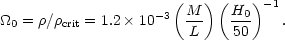
(3)

If H₀ = 50, M/L must be equal ~ 1000 for ₀ = 1 .

1.2.2    PREDICTION OF THE REDSHIFT DISTRIBUTION IN VARIOUS MAGNITUDES INTERVALS    Galaxies that appear within an apparent magnitude interval m ± 1/2 dm are spread in distance, and therefore in redshift, according to their distribution of absolute magnitudes (M). If (M) = (M), the galaxies that contribute to the interval dM at m are all within a distance range dr at r given by

(4)

and are therefore within the redshift interval

(5)

where H₀ is the Hubble constant. When (M) (M), but rather has a distribution of absolute magnitude, the number of galaxies in the magnitude range (m₁, m₂) at velocity v in interval dv in solid angle w is given by

(6)

where D is the number of galaxies per cubic megaparsec at the distance r = 10^{0.2(m - M - 5)}. Equation 6 can be used, for example, to calculate the expected redshift distribution of a complete sample of galaxies between, say, apparent magnitudes m - 0.5 and m + 0.5. The equation assumes Euclidean geometry and is valid therefore for low velocities (z 0.5). Proper volumes for various q₀ values must be used in the general case (cf. Section 1.2.4).

An example of predicted velocity distributions for galaxies between m = 10 and m = 11 up to m = 14 to m = 15 using the general luminosity function given by Tammann et al. (1979; hereinafter TYS) has been calculated by Schweizer (1987, Figure 12). The observed redshift distributions for very faint galaxies have been summarized by Ellis (1987) and Koo & Kron (1987) for two narrow pencil-beam surveys to B ~ 21 and B ~ 22, respectively. The decided nonuniformity in both distributions is because the surveys cut through the boundaries of sheets and voids along the line of sight. An accurate calculation of the expected envelope of the distribution requires knowledge of (M), the K correction (see Section 2), and luminosity evolution at each look-back time.

1.2.3    PREDICTED SURFACE DENSITY OF dE DWARFS THAT WILL BE BRIGEITER THAN APPARENT MAGNITUDE m    Biased galaxy formation requires that the giant-to-dwarf ratio be a function of the mean density. Faint galaxies should exist in the low-density regions, but giants should be absent. On the other hand, if dwarf galaxies can only form as satellites of giants, the giant-to-dwarf ratio should not depend on environmental density. A search for dwarf galaxies in the general field (Binggeli et al. 1988) can address this problem of the shape of (M) depending on density. Predictions of the expected surface density of dwarfs indicate what such a survey might find.

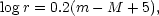
The number of galaxies per square degree that should be present in the apparent magnitude interval dm at m, contributed from the absolute luminosity interval M₁ to M₂, is

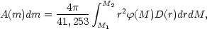
(7)

where m, M, and r are related by m - M + 5 = 5log r. [The number of square degrees in the sky is 4(180 / )² = 41, 253.]

The most illuminating way to solve Equation 7 is to replace the integral by a sum over discrete volume segments defined by inner and outer distances separated by logr = logr₂/r₁ = 0.2. This gives intervals of 1 mag in m - M. If (M) D(r) is tabulated for 1-mag intervals (such that M + 0.5 and M - 0.5 are the boundaries of the tabulation), A(m) will be the surface density of objects at m in the 1-mag interval m - 0.5 to m + 0.54 This procedure is the log method of solving Equation 7, originally due to J.C. Kapteyn and to F.H. Seares (cf. Bok 1936, Mihalas & Binney 1981). Applying Equation 7 with (M) from TYS (their Figure 3) and integrating over the dwarfs defined as galaxies fainter than M = - 15 gives a series of A(m) values for various assumptions of the slope of (M) at the faint end. For exponential increases in (M) given by log(M) = constant + am (fitted to the bright-end shape and normalization of TYS), summing the A(m) values to obtain N(m) gives the predicted number of dwarfs brighter than m = 17.5 and 18.5 per square degree whose absolute magnitudes are between -15 and -8 (Table 1). The third line of Table 1 gives the ratio of the number of dwarfs to the total number of galaxies (of all luminosities) and shows that only a few percent of a complete surface survey of galaxies are expected to be dwarfs.

Table 1. Expected N(m) per square degree for dwarfs fainter than M = - 15

	Slope values
mB	0.2	0.3	0.4
17.5	0.1	0.5	2.6
18.5	0.5	2.0	10.2
Percent of total	0.3	1	5

A more useful calculation of the expected numbers of dE and Im types taken separately requires knowledge of the specific luminosity function _T(M) for each of these types (Section 5).

1.2.4    THE COSMOLOGICAL N(m) TEST    Galaxy counts to faint magnitudes give A(m) and hence N(m) = A(m)dm. These observational data can be compared with calculated A(m) values using an equation similar to Equation 7. But there now is the complication of spatial curvature for the volume element. Also, the Mattig (1958) relation between m, M, and r must be used rather than m - M + 5 = 5log r. Luminosity evolution in the look-back time can be included by making (M) D(r) a function of r (or redshift, meaning time). Hence, the look-back time as a function of geometry must also be known. The K-correction (Section 2) also becomes very important and can be included in the _T(M, z) relations for various galaxy types.

No details of these complicated calculations have yet been given either in the literature or in textbooks, but the concepts are straightforward using the version of Equation 7 that takes non-Euclidean geometry into account.

Results (but not the details) of such calculations, with and without evolution, are given by Peterson et al. (1979), who also provide references for the pre-1979 literature. A review by Ellis (1987) gives more recent results.