


Consider the case in which a single physical quantity, y,
is some function of the  's:
y = y(1, ...,
M). The "best"
value for y is then y* =
y(i*).
For example y could be the path
radius of an electron circling in a uniform magnetic field where
the measured quantities are
1 =
's:
y = y(1, ...,
M). The "best"
value for y is then y* =
y(i*).
For example y could be the path
radius of an electron circling in a uniform magnetic field where
the measured quantities are
1 =
 , the period of revolution,
and
2 = v, the
electron velocity. Our goal is to find the
error in y given the errors in
. To first order in
(i -
i*) we have
, the period of revolution,
and
2 = v, the
electron velocity. Our goal is to find the
error in y given the errors in
. To first order in
(i -
i*) we have
| (12) |
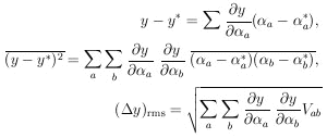
A well-known special case of Eq. (12), which holds only when the variables are completely uncorrelated, is
|
In the example of orbit radius in terms of
and v this becomes
|
in the case of uncorrelated errors. However, if
 is
non-zero as one might expect, then Eq. (12) gives
is
non-zero as one might expect, then Eq. (12) gives
|
It is a common problem to be interested in M physical parameters,
y1, ..., yM, which are known
functions of the
i.
In fact the yi can be thought of as a new set of
i or a
change of basis from
i to
yi. If the error matrix of the
i
is known, then we have

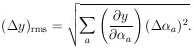
| (13) |
In some such cases the ðyi /
ða cannot be
obtained directly, but the
ði /
ðya are easily
obtainable. Then
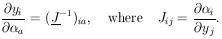
|
Example 3
Suppose one wishes to use radius and acceleration to
specify the circular orbit of an electron in a uniform magnetic
field; i.e., y1 = r and y2 =
a. Suppose the original measured quantities are
1 =
= (10 ± 1)µs and
2 = v =
(100 ± 2) km/s. Also
since the velocity measurement depended on the time measurement,
there was a correlated error
= 1.5 × 10⁻³
m. Find
r, r, a,
a.
r, a,
a.
Since r = v /
2 = 0.159 m and
a = 2v /
= 6.28 × 10¹⁰
m/s2 we have y1 =
12 /
2 and
y2 = 2
2 /
1. Then
ðy1 /
ð1 =
2 /
2,
ðy1 /
ð2 =
1 /
2,
ðy2 /
ð1 =
-22 /
12,
ðy2 /
ð2 =
2 /
1 . The
measurement errors specify the error matrix as
= 0.159 m and
a = 2v /
= 6.28 × 10¹⁰
m/s2 we have y1 =
12 /
2 and
y2 = 2
2 /
1. Then
ðy1 /
ð1 =
2 /
2,
ðy1 /
ð2 =
1 /
2,
ðy2 /
ð1 =
-22 /
12,
ðy2 /
ð2 =
2 /
1 . The
measurement errors specify the error matrix as
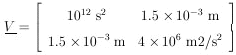
|
Eq. 13 gives
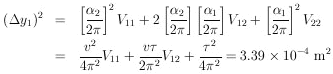
|
Thus r = (0.159 ± 0.184) m
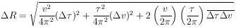
For y2, Eq. 13 gives

|
Thus a = (6.28 ± 0.54) × 1010 m/s2.