3.3. Isodelay Surfaces

Suppose for the moment that the BLR consists of clouds in a thin spherical shell of radius r. Further suppose that the continuum light curve is a simple -function outburst. Continuum photons stream radially outward and after travel time r/c, about 10% of these photons (using a typical "covering factor") are intercepted by BLR clouds and are reprocessed into emission-line photons. An observer at the central source will see the emission-line response from the entire BLR at a single instant with a time delay of 2r/c following the continuum outburst. At any other location, however, the summed light-travel time from central source to line-emitting cloud to observer will be different for each part of the BLR. In the case of a -function outburst, at any given instant, the parts of the BLR that the observer will see responding are all those for which this total path length is identical; at any given time delay, the part of the BLR that the observer sees responding is the intersection of the BLR distribution and an "isodelay surface." Astronomers, on account of their familiarity with conic sections, can readily recognize that the shape of the isodelay surface is an ellipsoid with the continuum source at one focus and the observer at the other; the light-travel time from central source to BLR cloud to observer is constant for all points on the ellipsoid. 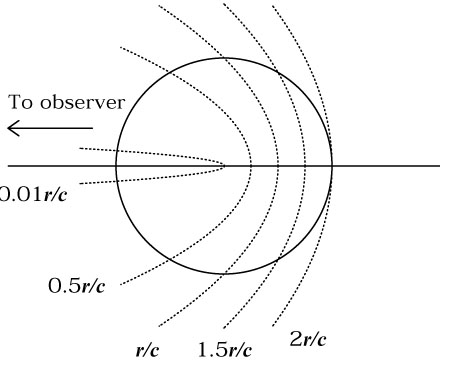Since the observer is virtually infinitely distant from the source, the isodelay surface becomes a paraboloid, as shown schematically in Fig. 6. The figure shows the BLR as a ring intersected by several isodelay surfaces, labeled in terms of their time delay in units of r/c. Relative to the continuum, points along the line of sight to the observer are not time delayed (i.e., = 0). Points on the far side of the BLR are delayed by as much as 2r/c, the time it takes continuum photons to reach the BLR plus the time it takes line photons emitted towards the observer to return to the central source on their way to the observer.

Figure 6. The circle represents a cross-section of a shell containing emission-line clouds. The continuum source is a point at the center of the shell. Following a continuum outburst, at any given time the observer far to the left sees the response of clouds along a surface of constant time delay, or isodelay surface. Here we show five isodelay surfaces, each one labeled with the time delay (in units of the shell radius r) we would observe relative to the continuum source. Points along the line of sight to the observer are seen to respond with zero time delay. The farthest point on the shell responds with a time delay 2r/c.

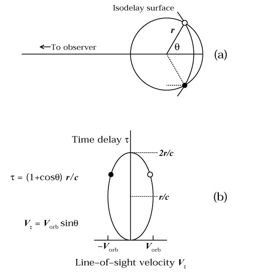
Figure 7. The upper diagram shows a ring (or cross-section of a thin shell) that contains line-emitting clouds, as in Fig. 6. An isodelay surface for an arbitrary time is given; the intersection of this surface and the ring shows the clouds that are observed to be responding at this particular time. The dotted line shows the additional light-travel time, relative to light from the continuum source, that signals reprocessed by the cloud into emission-line photons will incur (Eq. (23)). In the lower diagram, we project the ring of clouds onto the line-of-sight velocity/time-delay (Vz, ) plane, assuming that the emission-line clouds in the upper diagram are orbiting in a clockwise direction (so that the cloud represented by a filled circle is blueshifted and the cloud represented by an open circle is redshifted).

Essentially, the transfer function measures the amount of line emission emitted at a given Doppler shift in the direction of the observer as a function of time delay . The value of the transfer function at time delay is computed by summing the emission in the direction of the observer at the intersection of the BLR and the appropriate isodelay surface. For a thin spherical shell, the intersection of the BLR and an isodelay surface is a ring of radius r sin , where the polar angle is measured from the observer's line of sight to the central source, as shown in Fig. 7. The time delay for a particular isodelay surface is the equation for an ellipse in polar coordinates,

(23)

as is obvious from inspection of Fig. 7. The surface area of the ring of radius r sin and angular width r d is 2 (r sin) r d, and assuming that the line response per unit area on the spherical BLR has a constant value ₀, the response of the ring can be written as

(24)

where 0 2. From Eq. (23), we can write

(25)

so putting the response in terms of rather than , we obtain

(26)

for values from = 0 ( = 2) to = 2r/c ( = 0). The transfer function for a thin spherical shell is thus constant over the range 0 2r/c.