3.4. Transfer Functions for a Variety of Simple Models

The simple analytic calculation in the last section was intended to be illustrative and serve as a reference point. We will now expand on this with more general geometries, and also incorporate information from Doppler motion along the line of sight. We will derive some transfer functions for other simple models, focusing on three: (a) systems of clouds in circular Keplerian orbits, illuminated by an isotropic continuum, (b) biconical outflows, and (c) disks of random inclination. All these are physically plausible, and can produce "double-peaked" emission-line profiles, which are sometimes seen in AGNs, though not all of these models necessarily do this. We will start with the simplest models and progress to more complicated models. Much of this discussion is drawn from discussions of transfer functions in the literature ^{93, 60, 24, 30, 31} .

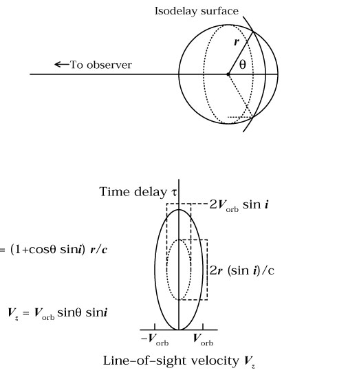
Suppose line-emitting clouds are on a circular orbit at inclination i = 90°; imagine that the circle in Fig. 7a represents this orbit seen face on. The line response from the clouds at the intersection of an arbitrary isodelay surface and the circular orbit will be at time delay = (1 + cos ) r/c and line-of-sight velocities V_z = ± V_orb sin, where V_orb = (GM / r)^1/2, the circular orbital speed. It is easy to see that the circular orbit projects to an ellipse in the line-of-sight velocity/time-delay (V_z, ) plane with semiaxes V_orb and r/c, as shown in Fig. 7b. This simple example is important because it is straightforward to generalize it to both disks (rings of different radii) and shells (rings at different inclinations).

First we consider the generalization to a shell. We can construct a shell from a distribution of circular orbits, with inclinations ranging from i = 0° to i = 180°. As we decrease the inclination of the circular orbit in Fig. 7a from i = 90°, we see that the range of time delays will decrease from [0, 2r/c] to [(1-sin i) r/c, (1 + sin i) r/c], and similarly the line-of-sight velocity range will decrease from [-V_orb, +V_orb] to [-V_orbsin i, +V_orbsin i], as we show schematically in Fig. 8. At the limiting case i = 0°, the time delays all contract to r/c, since the light travel-time paths for all points on a face-on ring are the same, and the velocities all contract to V_z = 0, because the orbital velocities are now perpendicular to the line of sight. Thus, the transfer function looks like a series of ellipses as in Fig. 8b that with decreasing inclination contract down to a single point at V_z = 0 and = r/c when i = 0°. We can construct such a transfer function by using a Monte Carlo method that places BLR clouds randomly across the surface of the shell, and the result we get is shown in Fig. 9, which corresponds to a thin shell of radius 10 light days and a central mass of 10⁸ M. We have also integrated this transfer function over and V_z to obtain the emission-line profile and the one-dimensional transfer function, respectively. In the particular case of a thin spherical shell, we see that both of these are simple rectangular functions, as we showed analytically for the one-dimensional transfer function (Eq. (26)).

Figure 8. Here we take the circular ring shown in Fig. 7 and show how its projection on Vz, changes as the inclination is decreased from 90°; in the time-delay direction, the axis contracts to 2r sin i / c, and in the velocity direction it decreases to 2Vorb sin i.

The first complication that we might consider is anisotropic line emission by the BLR clouds. Physically, this will occur if the BLR clouds themselves are optically thick in the lines as well as the continuum. In this case, most of the line radiation emitted by the clouds will be from the side of the cloud facing the continuum source, i.e., the line emission is directed back towards the continuum source. A simple parameterization of asymmetric line emission is to describe the apparent emissivity of a cloud as

(27)

where ₀ is constant and the parameter A = 0 for isotropic emission and A = 1 for completely anisotropic emission; the latter case is appropriate for spherical clouds with inward-facing surfaces that are uniformly bright. In principle, A can be estimated by photoionization modeling, though in practice the values are highly uncertain on account of limitations in the accuracy of the radiative transfer codes (see the contribution by Netzer). It is certainly expected that A 1 for Ly, at least, and models suggest approximate values A 0.7 for C IV and A 0.8 for H 24 . The main effect of anisotropic emission is to increase the measured lag for a given geometry because the apparent response of the near side of the BLR is suppressed. For a thin shell of radius r, the mean time delay is = (1 + A / 3) r/c. Fig. 10 shows the transfer function for the same thin spherical shell model of Fig. 9, but in this case with highly anisotropic (A = 1) line response.

Figure 9. Transfer function for a thin spherical shell. The upper left panel shows in grey scale the two-dimensional transfer function, i.e., the observed emission-line response as a function of line-of-sight velocity Vz and time delay . The upper right panel shows the one-dimensional transfer function, i.e., the two-dimensional transfer function integrated over Vz, which is the response of the total emission line as a function of time (cf. Eq. (26)). The lower left panel shows the emission-line response integrated over time delay; this is the profile of the variable part of the line. The specific model here is comprised of emission-line clouds in circular orbits of radius r = 10 light days and random inclinations (0° i 180°), orbiting around a central black hole of mass 108 M. In this model, the line emission from each cloud is isotropic (A = 0).

Figure 10. Transfer function for a thin spherical shell, as in Fig. 9, except with completely anisotropic (A = 1) line emission, i.e., all of the emission line flux from each cloud is directed back towards the continuum source.

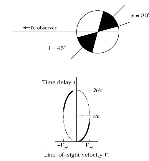
In addition to anisotropic line response, we can also consider anisotropic illumination of the BLR clouds by the continuum source. As an example, consider the case where BLR clouds are illuminated by biconical beams of semi-opening angle ; the limiting case as approaches zero would be a narrow jet-like pencil beam, and the case = 90° corresponds to an isotropic continuum. We start by examining the response of an edge-on (i = 0°) circular ring, as we show in Fig. 11, which is exactly like Fig. 7, but with only part of each orbit illuminated by the continuum source. We earlier generalized the result for a shell, going from to Fig. 8 as we decreased the inclination of the ring; doing this again, we see in Fig. 12 how the two-dimensional transfer function is altered by anisotropic illumination. We note specifically the absence of any response near = 0 and = 2r/c since the bicones shown do not illuminate BLR clouds directly along the observer's axis. Similarly there is also no response around = r/c due to the absence of response of clouds at 90°.

Figure 11. A ring-like line-emitting region and its projection into the Vz, plane is shown, as in Figs. 7 and 8, though in this case with a biconical continuum geometry. In the case shown here, the beam semi-opening angle is = 30°, and the beam is inclined to the observer by i = 45°. Again assuming that clouds on the ring are orbiting in the clockwise direction, we highlight in the lower diagram the regions in the (Vz, ) plane that will produce an emission-line response; there is no emission-line response from clouds not illuminated by the continuum beam.

So far we have restricted our attention to "thin" geometries, i.e., single orbits and shells. Generalization to "thick" geometries, e.g., disks and shells with different inner and outer radii, is trivial: the response of a disk can be computed by integrating over a series of circular orbits, and the response of a thick shell is obtained by integrating over a series of shells. In Fig. 13, we illustrate this concept by showing the response from two rings.

Figure 12. Transfer function for a thin spherical shell, as in Fig. 9, except with an anisotropic continuum source. In the example shown, the beam opening angle is = 30° and the inclination is i = 45°, as in Fig. 11.

Figure 13. Two ring-like regions (as in Fig. 7), and their projected response on the (Vz, ) plane.

Thus far, the free parameters we have dealt with are the radius r, the line anisotropy factor A, and in the case of non-spherically symmetric systems, the inclination i and, in the case of biconical illumination, the beam half-angle . Thick geometries now introduce inner and outer radii, r_in and r_out, respectively, and a distance-dependent responsivity per unit volume (or per unit area, for a disk), which we can parameterize as (r) ₀ r. The index allows us to condense model-dependence into a single parameter that will account for effects due to geometrical r^-2 dilution of the continuum, a distance-dependent covering factor, etc. In Figs. 14 and 15 we show transfer functions for thick spherical shell systems with A = 0 and identical values of r_in and r_out, but differing radial-response indices ; the effect of increasing is to enhance the relative response of material at larger radii; the limiting cases where -> - and -> + correspond to the response functions of thin shells of radius r_in and r_out, respectively. We will show additional examples below.

Figure 14. Transfer function for a thick spherical shell with rin = 2 lt-days, rout = 10 lt-days, and radial responsivity index = 0.

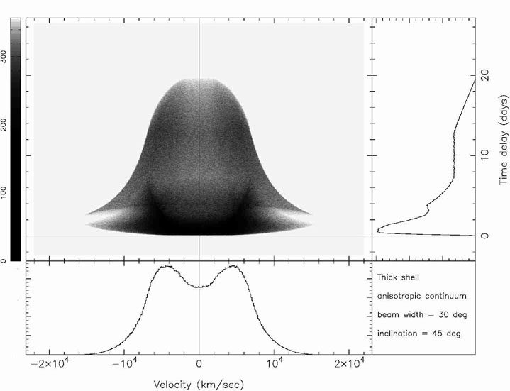
We consider now a thick shell system that is illuminated by an anisotropic continuum source. Again, we assume that the line-emitting clouds are in circular Keplerian orbits of random inclination. We show examples that are identical except for the continuum beam width and inclination in Figs. 16 and 17. An important thing to notice is that in one case (Fig. 16) the observer is outside of the continuum beam (i.e., i > ) and in the other case (Fig. 17) the observer is inside of the continuum beam (i.e., i < ); when the observer is inside the beam, the line profile is single-peaked, and when the observer is outside the beam, the line profile is double-peaked.

Figure 15. Transfer function for a thick spherical shell exactly as described in Fig. 14, except with radial responsivity index = -4.

Figure 16. Transfer function for a thick spherical shell with rin = 2 lt-days, rout = 10 lt-days, radial responsivity index = -2, and isotropic line response A = 0. In this model, the shell is illuminated by a biconical continuum with semi-opening angle = 30° and inclination i = 45°, i.e., the observer is outside the continuum beam. Note the double-peaked line profile, and contrast this with the model shown in Fig. 17.

Figure 17. Transfer function for a thick spherical shell exactly as described in Fig. 16, except that in this model the shell is illuminated by a biconical continuum with semi-opening angle = 75° and inclination i = 15°, i.e., the observer is well inside the continuum beam. Note the single-peaked line profile, and contrast this with the model shown in Fig. 16.

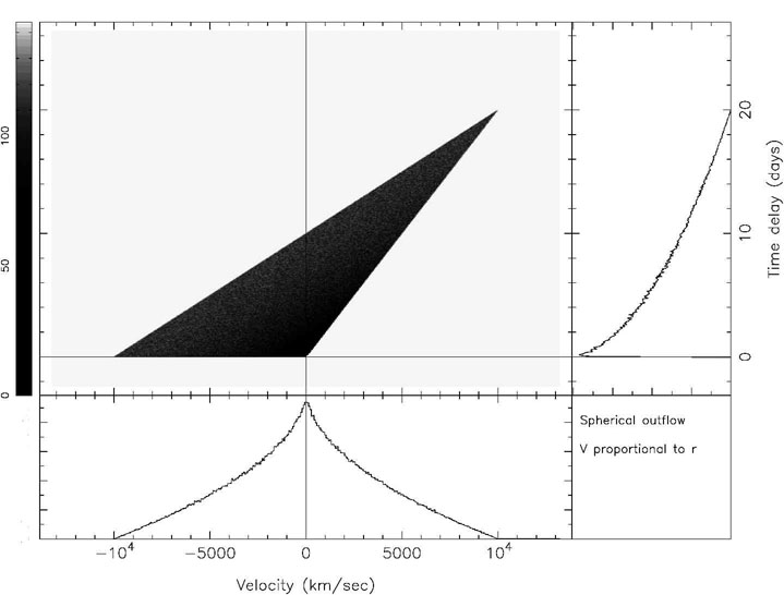
Another simple kinematic model for the BLR consists of clouds in spherical outflow. The transfer functions for such cases are quite distinctive; an example of a two-dimensional tranfer function for a kinematic field with radial velocity V_r r for r less than some maximum distance r_out is shown in Fig. 18. This velocity field corresponds to either a ballistic outflow or a flow undergoing constant acceleration. At = 0 we see response from all the material along the line of sight to the continuum source, which ranges from V_z = 0 for the material closest to the central source to V_z = -V(r_out) for the gas farthest from the continuum source. As increases, we begin to see response from the far side of the BLR where the line of sight velocities V_z become positive. The range of line-of-sight velocities decreases as the isodelay surfaces get farther from the line of sight. At = r_out / 2, the isodelay surface no longer crosses any clouds moving towards the observer, and the gas moving fastest away from the observer is that along the line of sight ( = 0) with V_z = V(r_out) / 2. At = 2r_out / c, only the response from the antipodal point is seen, and the transfer function is contracted to the single point at [2r_out / c, V(r_out)].

Figure 18. Transfer function for a spherical outflow, with outflow velocity V r. For this model, rin = 0.1 lt-days, rout = 10 lt-days, V(rout) = 10000 km s-1.

The case of biconical outflows (which are possibly relevant, as they are certainly seen in the NLR and might well apply to at least a component of the BLR) can be dealt with by restricting the response to certain values of ; an example is shown in Fig. 19.

Figure 19. Transfer function for a biconical outflow, with parameters as in Fig. 18 except that the outflowing gas is confined to a bicone of half-width = 30° at inclination i = 45°.

We have now seen that both orbital and outflow models can produce similar emission-line profiles; if the line-emitting gas is confined to a bicone, either because of the gas distribution or the ionizing-photon distribution, one can get a single-peaked or double-peaked line profile. The two situations can be easily distinguished, however, by their two-dimensional transfer functions (or equivalently, the combination of their one-dimensional transfer functions and their line profiles). In Fig. 20, we directly compare the one-dimensional transfer functions and line profiles for two thick-shell models: (1) emission-line clouds in a biconical outflow and (2) clouds in circular Keplerian orbits of random inclination, illuminated by a biconical continuum source. In both cases, the beams (one radiation, one matter) have the same half-opening angle ( = 40°) and two different inclinations are shown; i = 25° in the top row (i.e. the observer is in the beam, as indicated in the left-hand column illustrations of the geometry), and i = 65° in the bottom row (i.e., the observer is out of the beam). The distribution of line-emitting clouds is the same, regardless of how the clouds are moving, so in these two cases the one-dimensional transfer functions ought to be very similar, which is indeed the case, as seen in the middle column of Fig. 20. The right-hand column shows the line profiles, which are however very different. Consider the case i = 25° (top row): in the case of outflow, the line-emitting material in the beam is moving radially outward, giving relatively highly blueshifted (near side) and redshifted (far side) emission, but little emission near V_z = 0, since there is no line-emitting material moving transverse to the line of sight. In the case of clouds in circular orbits illuminated by an anisotropic beam, the cloud motions are perpendicular to their radial vectors, so most of the line-emitting material is at low Doppler shift as the gas motions through the beams are predominantly transverse. Now consider the higher-inclination case (i = 65°; bottom row): in the case of radial outflow, the gas motions in this case are now primarily transverse so the Doppler shifts are smaller. However, in the case of circular orbits, the material in the beam is moving primarily along the line of sight, and there is a deficiency of material at V_z 0.

Figure 20. Response of two biconical models with different kinematics. The left hand column shows the two geometries considered, both with beam half-opening angles = 40°; the top row is at inclination i = 25° (i.e., the observer is in the beam) and the bottom row is i = 65° (i.e., the observer is out of the beam). One-dimensional transfer functions (middle column) and line profiles (right column) are shown. The solid line is a biconical outflow model, and the dashed line represents circular Keplerian orbits of random inclination. The one-dimensional transfer functions are identical, but the profiles are greatly different, as described in the text.

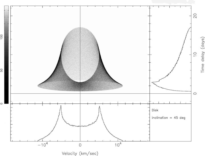
Finally, for completeness, we consider the case of an inclined disk, as this is the classic geometry for producing a double-peaked line profile. The response of a disk-like BLR can be computed by integrating the response of rings of different radii. In Fig. 21, we show the transfer function and line profile for a disk at intermediate inclination (i = 45°). Identical line profiles can be obtained for different inclinations simply by suitably adjusting the central mass, but the transfer function allows us to reduce the ambiguity between possible disk models.

Figure 21. Transfer function for a thin disk at intermediate inclination (i = 45°). Note that the line profile is double peaked, and the one-dimensional transfer function is similar to those for spherical shells.