


4.3. Discrete Correlation Methods
There are some circumstances under which one might not
be able to reasonably interpolate between gaps in data.
This can occur (a) when there are a few large gaps in
otherwise well-sampled series or (b) when there is reason
to believe that the variations might be at least somewhat
undersampled. In these cases, interpolation might be
highly misleading, and another methodology needs to be
employed. The "discrete correlation function" (DCF)
20
method is one where no assumption about light curve behavior
needs to be made. The DCF method deals with irregularly
sampled data by binning the data in time, as illustrated
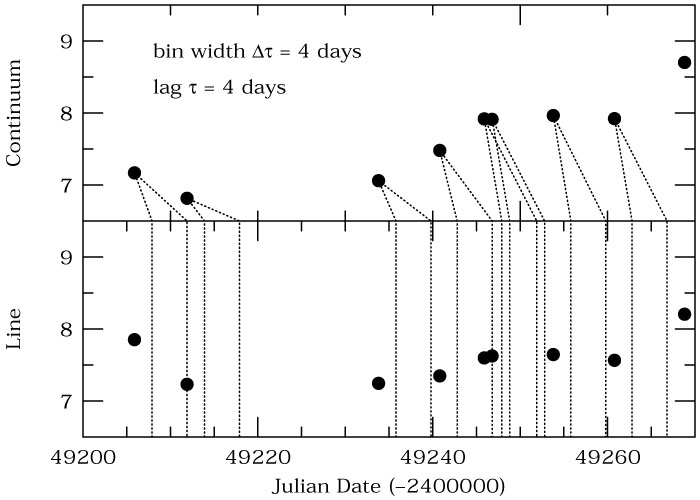
schematically in Fig. 27. This is an
alternative approach to the irregular sampling requirement:
instead of requiring that points contributing to
CCF( ) are separated in time by
exactly the interval , we
time-bin the data by pairing points with time separations in the range
±
) are separated in time by
exactly the interval , we
time-bin the data by pairing points with time separations in the range
±
 / 2, where
is
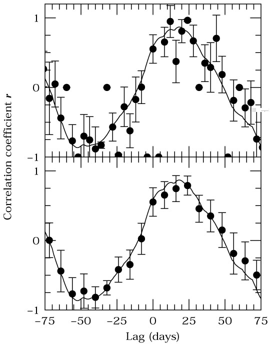
the width of one time bin. Choice of the
binning window is a free parameter, and two examples
are shown in Fig. 28.
/ 2, where
is
the width of one time bin. Choice of the
binning window is a free parameter, and two examples
are shown in Fig. 28.
|
Figure 27. Part of the light curves from
the previous figures,
expanded to show DCF bins. The particular example shown is
for a time-lag bin width
|
|
Figure 28. Cross-correlation functions for the
Mrk 335 light curve shown in Fig. 23.
The DCF values are shown as points with error bars,
and the interpolation CCF, as in
Fig. 25,
is shown as a solid line. The upper panel shows the
DCF with a bin width of |
The principal virtues of the DCF method are (a) that only actual data points are used and (b) that it is possible to assign a statistical uncertainty to the value of the correlation coefficient in each bin. The relative weakness of the DCF is that the data are in some ways underutilized, as is evident in Fig. 27; for a small data set, the DCF method might completely miss a real correlation, although it is less like to find a spurious correlation than is the interpolation method 94.
One difficulty of the DCF method is that the number of points per time bin can vary greatly, as can be easily inferred from inspection of Figs. 27 and 28. One solution to this is to vary the width of the time bins to ensure that there are a statistically meaningful number of points in each bin. A method for accomplishing this is the "Z-transformed DCF (ZDCF)" 1.