© CAMBRIDGE UNIVERSITY PRESS 2000

22.2. Spherical isotropic models

For systems such as globular clusters it is natural to look for a description in terms of a distribution function dependent only on the energy E = v²/2 + (r). For these small stellar systems, it is plausible that they have moved significantly in the direction of a relaxed quasi-Maxwellian, with a truncation radius provided by the tidal environment where the globular cluster moves. This is the basic physical motivation for solutions of the type described in the following section. It should be stressed that the main success of these truncated models is that they can indeed provide a physically based description of the global structure of an important class of stellar systems. For comparison, we will later describe the classical isothermal sphere (which has infinite mass) and other tools (models obtained via adiabatic deformations) that find their best applications to the local structure of the cores of stellar systems.

22.2.1. Global truncated (King) models

Consider a spherical distribution of stars f = f (E) limited to a sphere of radius r_t. The collection of stellar orbits described by f is thus subject to the condition that f vanishes for E > (r_t). Suppose that the distribution function has the following form

(22.5)

for E < (r_t) (and f = 0 otherwise). Here A, a, and r_t are free constants, defining two scales and one dimensionless parameter. We may introduce the dimensionless "escape" energy defined as

(22.6)

Thus the condition E < (r_t) can be written as av²/2 < . The density profile (for r < r_t, i.e. > 0) associated with the distribution function is given by

(22.7)

By a simple change of integration variables the density can be written as

(22.8)

with

(22.9)

where is the incomplete Gamma function ⁽²⁶⁾. Note that the density, in this isotropic model, depends on the radial coordinate only implicitly through the potential (r). For large values of we have ~ (3^1/2/4) exp(), i.e. it behaves like the density of non-truncated isothermal models (see following section).

By a suitable rescaling of the radial coordinate r = r / the self-consistency relation implied by the Poisson equation can thus be written as

(22.10)

which is to be integrated subject to the boundary conditions (0) = > 0 and '(0) = 0. Thus the scalelength can be defined in terms of the central density ₀ and of the dimensionless depth of the central potential well by means of the relation

(22.11)

Close to the center the potential well can be approximated by a parabola with

(22.12)

Integrating Eq. (10) out determines the radius r_t as the location where vanishes. Thus a one-to-one correspondence is found between and r_t / . A commonly used scalelength for this problem is

(22.13)

The one-parameter family of models, usually called King models ⁽²⁷⁾ (see Figs. 22.1 - 22.3), is thus identified either by the value of or, more often, by the value of the concentration index

(22.14)

As a model for elliptical galaxies ⁽²⁸⁾, the required concentration parameter is in the range 2 < C < 2.35, although the R^1/4 profile is not reproduced in detail. Highly concentrated King models (formally C ) go in the direction of the isothermal sphere to be described below. It should be stressed that, in spite of a being a constant, the velocity dispersion associated with the distribution function of Eq. (5) is not a constant. The velocity dispersion monotonically decreases with radius and vanishes at the truncation radius (see Fig. 22.4).

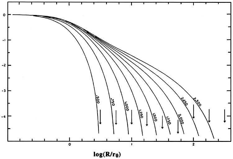Figure 22.1. Projected density profiles for the King models (from King, I.R. 1967, Vol. 9 of the AMS Lectures in Applied Mathematics, Relativity Theory and Astrophysics 2. Galactic Structure, ed. J. Ehlers, American Mathematical Society, Providence, RI p.116). The curves show the logarithm of the projected density (normalized to the central value) for selected values of the concentration parameter C (marked along the curves). For each case an arrow provides the location of the relevant truncation radius rt.

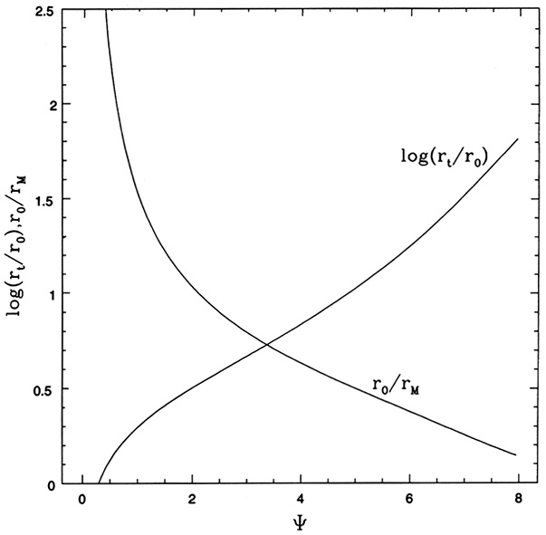Figure 22.2. Concentration parameter C and scale r0 relative to the half-mass radius rM as a function of the central dimensionless potential for King models (adapted from Vesperini, E. 1994, Ph.D. Thesis, Scuola Normale Superiore, Pisa, Italy).

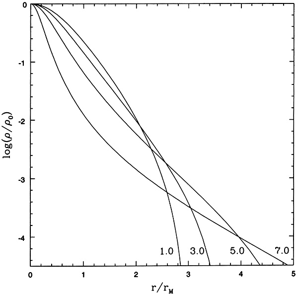Figure 22.3. Density profiles for selected values of the central dimensionless potential ( = 1, 3, 5, 7) for King models (adapted from Vesperini, E. 1994, Ph.D. Thesis, Scuola Normale Superiore, Pisa, Italy).

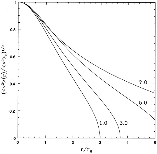Figure 22.4. Velocity-dispersion profiles for selected values of the central dimensionless potential ( = 1, 3, 5, 7) for King models (adapted from Vesperini, E. 1994, Ph.D. Thesis, Scuola Normale Superiore, Pisa, Italy).

The radius r₀ is sometimes confused with the "core radius" r_c of the projected density distribution, usually defined as the location where the projected density has dropped to one half of its central value. With the definition of Eq. (13) the identification is correct for the isothermal sphere (see below), and it is reasonable for concentrated King models ⁽²⁹⁾, while at lower values of the ratio r₀/r_c changes significantly with .

Applications of these models to globular clusters have been very successful. The globular clusters of our Galaxy ⁽³⁰⁾ are generally well fitted by King models with concentration parameter in the range 0.5 < C < 2 (see Fig. 22.5); some are even more concentrated, but they are generally considered to be in a "post-core-collapse" phase, since the onset of the gravitational catastrophe ⁽³¹⁾ is known to take place at 7.4. One can take full advantage of the equilibrium sequence by arguing that the identifying parameters (total mass, central velocity dispersion, and concentration) can change as a result of evolutionary processes (such as evaporation and disk-shocking), while the underlying model retains its King appearance ⁽³²⁾. By this representation it is possible to follow the evolution of a whole population of globular clusters in a galaxy with a rather handy algorithm ⁽³³⁾, thus clarifying many of the interesting correlations in the relevant parameter space observed for the clusters of our Galaxy.

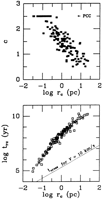Figure 22.5. Empirically determined dynamical properties of globular clusters in the Milky Way (from Djorgovski, S., Meylan, G. 1994, Astron. J., 108, 1292). Above: Concentration parameter vs. core radius; post-core-collapse clusters are assigned the value C = 2.5. Below: The value of the central relaxation time trc, estimated on the basis of the empirically determined central properties of the clusters (see Chapter 7). The apparent strong correlation with the core radius just reflects the operational definition of trc.

22.2.2. The isothermal sphere

We now consider the spherical analogue of the isothermal slab solution described in section 14.1 (in the context of the vertical equilibrium of a disk). That calculation was especially instructive, as a very simple case of a stellar dynamical study with distribution function priority. We may recall that the isothermal slab implied a constant gravity field at large distances from the plane [see Eq. (14.9)], so that, as a model of a galaxy disk, its interest was mostly for a self-consistent description of the vicinity of the equatorial plane.

Similarly, besides its general interest as indicative of the divergences intrinsic to the hypothesis of a fully relaxed stellar system, the spherical solution to be described below provides a useful representation of the local behavior of many stellar systems in their central regions. It can clarify some of the properties of the more physical King models (which have been successfully applied to the interpretation of the global luminosity profiles of globular clusters). In addition, it also turns out to describe much of the structure inside the half mass radius of the partially relaxed, finite mass models that will be found to incorporate the R^1/4 profile (to be described in section 22.3).

If we take the distribution function

(22.15)

with no restrictions on the star velocities, we get an isothermal equation of state given by

(22.16)

with

(22.17)

Here we have introduced the dimensionless potential = -a (r). Note that the two constants A and a are dimensional parameters that may be used in order to match some physical scales of the system under investigation (e.g., the radius and the central velocity dispersion in the core of a galaxy). In contrast with the King models, there are no free dimensionless parameters available here. These relations are in analogy to those of section 14.1.1 and should be compared with the corresponding equations of the previous section. The fully self-consistent problem requires the solution of the Poisson equation

(22.18)

The scalelength is defined via the relation [see Eq. (11)]

(22.19)

If we look for a solution with finite central density the natural boundary conditions are (0) = and '(0) = 0. Since no free dimensionless parameters are available, here we can choose the value of in such a way that = r₀ (see Eq. (13). As is well known in studies of polytropic stars, the isothermal solution beyond the scale r₀ becomes asymptotically close to ~ r^-2, thus leading to an integrated mass increasing linearly with radius and making it inapplicable to describe the global profiles of stellar systems.

In the central regions [basically at radii r = O(r₀)], the density profile that is obtained numerically, when projected along the line-of-sight is found to match the general behavior of galaxy cores. The projected density (here R denotes the projected radius) is very close to the so-called modified Hubble profile

(22.20)

which can be traced to a volume density profile ⁽³⁴⁾ of the form

(22.21)

Obviously, the latter expressions find frequent applications because of their analytical simplicity.

One special solution with a singularity at the center is obtained when the condition of finite central density is dropped. This singular isothermal sphere corresponds to = -2 ln( / 2^1/2), which solves Eq. (18) exactly. Here the model loses the chacterization in terms of the central density and becomes "self-similar". The constants A and a are related to the constants b and V₀ of the logarithmic spherical mass model of section 21.1.3 via the relations a = 2/V₀² and b = 2^1/2 , with given by Eq. (19). The singular isothermal sphere presents close analogies with the isothermal self-similar disk described in section 14.3.2, in relation to the logarithmic potential that is found and to the type of divergences occurring at small and large radii. For the associated orbit structure we may thus refer to section 21.1.3.

Historically, the study of the isothermal sphere finds its roots in the theory of stellar structure, in relation to the Lane-Emden equation for polytropic star models ⁽³⁵⁾. We recall that the isotropic distribution function f = A(- E)^s for E < 0 (and f = 0 otherwise), with = 0 defining the surface of the associated stellar system, generates a density distribution (r) = B[- (r)]^s+3/2. Here A, B are constants. The Poisson equation thus becomes the same as the equation for a polytropic sphere ⁽³⁶⁾ with index n = s + 3/2. For the latter equation analytical solutions are known for n = 0, 1, 5. The case with n = 5 (with infinite radius) is often considered for its simple analytical structure ⁽³⁷⁾. In particular the associated Plummer density-potential pair is given by

(22.22)

(22.23)

The integrated mass is given by

(22.24)

so that the half-mass radius occurs at r_M 1.3b. The mean-square velocity is exactly <v²> = -(r) / 2 and the projected density is given by

(22.25)

22.2.3. Galaxy cores and anisotropic models obtained via adiabatic growth

We have noted at the beginning of the previous subsection that different emphasis can be given to the global or to a local application of stellar dynamical models. On the small scale (r << r_M) many models, such as King models or the ones that will be introduced in section 22.3, are characterized by a quasi-isothermal core, in the sense that they behave approximately as the (regular) isothermal sphere of section 22.2.2. On the other hand nuclei of galaxies have long been suspected to host massive point-like density concentrations (possibly black holes). It is thus of great interest to see whether adequate self-consistent models can be constructed where the field is due to the sum of the contributions of the stellar system and of a central point-mass. Clearly a comparison of the properties of these models with high resolution photometric and spectroscopic observations should eventually tell which galaxies host a central massive "black hole" and which do not. Major projects have been undertaken in the last few years focusing on these issues ⁽³⁸⁾. Either by means of stellar dynamical studies alone (in particular, for disk galaxies, such as M 31, NGC 3115, NGC 4594, our Galaxy, and for ellipticals ⁽³⁹⁾, such as M 32 and NGC 3377) or with the help of kinematical data from gas orbiting close to the central nucleus (see the spectacular cases of the giant elliptical M 87 and of the spiral galaxy NGC 4258 = M 106; see Fig. 22.6) convincing evidence has been accumulating for central black holes with masses in the range 2 × 10⁶ - 3 × 10⁹ M.

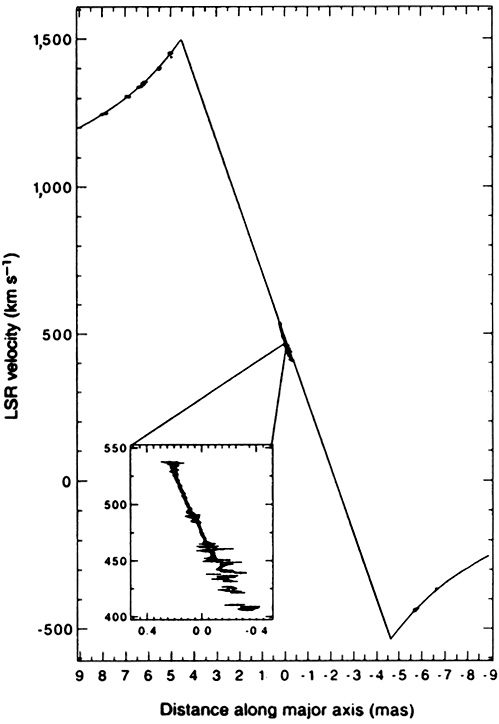Figure 22.6. A radio observation suggesting the presence of a massive black hole at the center of the galaxy M 106 (Fig. 3 from Miyoshi, M., Moran, J., Herrnstein, J., Greenhill, L., et al. 1995, Nature (London), 373, 127). The plot gives the line-of-sight velocity as a function of radial distance (in milliarcseconds) from the center, along the major axis of the observed molecular disk, with data superimposed on a model curve described in the cited paper. At the distance of the object (estimated to be 6.4 Mpc), 8 mas define a length of 0.25 pc.

Kinematical data are probably crucial to decide whether a central point-mass exists. Still it has been noted that, in the innermost regions (where the R^1/4-like profile is usually smeared out by seeing from the ground ⁽⁴⁰⁾), in some cases the luminosity profile, when studied at sufficiently high spatial resolution, does flatten out into a core structure, while in others the profile increases basically as a power-law ⁽⁴¹⁾, as far in as it is possible to observe. With the aid of the Hubble Space Telescope, for a sample of dozens of ellipticals (and bulges) this behavior has been traced down to a scale of 1pc from the center. Curiously, some of the parameters that characterize the galactic nuclear regions are found to correlate strongly with more global parameters.

In this short subsection we will not go further into this fascinating subject, but we will restrict our attention to some modeling issues that are found to be interesting because of their simple physical motivation. In contrast to the case without a central point mass, for which a core structure is naturally expected, in the presence of a 1/r singularity in the potential the stellar system should display a central cusp in its density distribution. In a study of this type, one important parameter is clearly the ratio M / M_c of the mass of the "black hole" to the mass of the core of the large-scale stellar density distribution.

Originally, much of the attention was drawn to the case of a black hole inside a collisional environment, such as that at the center of a globular cluster. Steady-state solutions of the Fokker-Planck equation were sought and constructed, thus applicable to timescales longer than the relevant two-body relaxation time ⁽⁴²⁾. In the regime of small masses of the central black hole, under the assumption that binary stars are unimportant, the cusp that is found is approximately given by ~ r^-7/4. In the following years, motivated by some of the observational studies mentioned above, the attention changed to the case of the more collisionless galaxy cores. A recent revival of interest in collisional steady-state solutions ⁽⁴³⁾ is motivated by the fact that one may imagine even the center of a galaxy to produce a collisional cusp via merging of small star clumps.

The collisionless case suggests the likely presence of significant anisotropies very close to the central point mass. There radial orbits would feel selectively the influence of the central singularity. A first simple study can be performed by focusing on the region outside such a black hole dominated environment and can be obtained in terms of the so-called "loaded polytropes" ⁽⁴⁴⁾. The basic idea is to see in such an outer region how the Lane-Emden equation is modified, thus reducing the discussion to that of a modified (isotropic) hydrostatic equilibrium with an assumed equation of state. One interesting finding of this much simplified description has been to show that a cusp structure forms, with properties that depend little on the polytropic index.

A more elegant construction of self-consistent stellar dynamical models can be made under the assumption that the central black hole grows slowly (on a time much longer than the relevant dynamical timescale) inside a pre-existing collisionless stellar system (thus on a time shorter than the relaxation time). In a spherical adiabatic growth ⁽⁴⁵⁾ the orbits associated with the distribution function are modified but conserve their angular momentum and their radial action. The process thus shows in a very intuitive way how anisotropy can be generated out of an initially isotropic system by the growth of the central mass.

Without entering in all the details, we would like to record here the structure of the equations that describe spherical adiabatic evolution. Suppose we separate the potential in two parts, so that the energy integral is given by

(22.26)

Here _ext⁰ is an external potential, while ⁰ is the self-consistent potential generated by the density associated with the distribution function f₀(E, J) describing the stellar system. We recall that the radial action J_r is defined as

(22.27)

the function v_r and the integral between the two turning points depend on the sum of the external and of the self-consistent potentials.

Now we can imagine that the external potential be varied slowly, by changing one parameter from its initial value ₀, so that it becomes _ext(r). This change will induce a change in the self-consistent potential from ⁰(r) to (r). In this slow process the radial action and the angular momentum are conserved, while the energy is not. So we may imagine to start from an orbit characterized by (E⁽⁰⁾, J) in the potential ⁰(r) + _ext⁰(r) and arrive at an orbit characterized by (E, J) in the potential (r) + _ext(r) with the condition:

(22.28)

This relation should be interpreted as a mapping between the "initial" value of the energy E⁽⁰⁾ and the "final" value of the energy E required for the radial action to remain constant. In other words this gives implicitly a relation E⁽⁰⁾ = E⁽⁰⁾(E, J). If we start from a distribution of stellar orbits f₀, the final distribution function will thus be given by

(22.29)

with E⁽⁰⁾ determined from Eq. (28). Self-consistency requires

(22.30)

These non-linear equations can be solved numerically (e.g., by iteration procedures) to derive the effects of adiabatic evolution. In particular one may consider the situation where _ext⁰ = 0 and f₀ = f₀(E) describes a non-singular isothermal sphere [see Eq. (15)], and ask what will be the final distribution function f (E, J) for _ext = - G M / r. The influence radius of the black hole is thus given by r = aG M, while the mass of the core can be defined from r₀ = aGM_c. The density cusp is found to be characterized by ~ r^-3/2 and associated with a kinematical cusp <v²> ~ G M / r. For a small black hole the density cusp emerges from the core region, while for large black holes the transition to the outer ~ r^-2 isothermal behavior occurs via an intermediate ~ r^-5/2 profile, with no distinct core left (see Fig. 22.7). The cusp is quasi-isotropic, with a small tangential bias at intermediate radii. These conclusions are changed if one starts from initial functions significantly different from that of the non-singular isothermal sphere. The extension to the case where some rotation and flattening are present is not trivial.

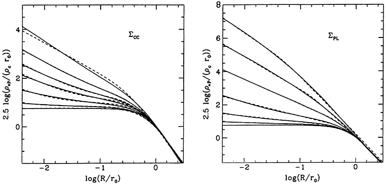Figure 22.7. Projected density cusps for models with a central black hole grown adiabatically onto an initial isothermal sphere are shown as solid lines (the central black hole mass values are 0, 0.03, 0.1, 0.2, 0.3, 0.5 (left) and 0, 0.03, 0.1, 0.3, 1, 3, 10 (right) in units of the core mass Mc). These dynamical model curves are shown here fitted by analytically simple formulas (dashed curves) introduced by Crane, P., Stiavelli, M., King, I.R., Deharveng, J.M., et al. (1993, Astron. J., 106, 1371) to fit the central photometric profiles of elliptical galaxies obtained from Hubble Space Telescope observations. (from Cipollina, M., Bertin, G. 1994, Astron. Astrophys., 288, 43).

Part of the structure of the solutions obtained by adiabatic growth can be clarified analytically. For this purpose one may refer to regions of phase space where the actions in the key mapping relation (28) can be approximated analytically (see Chapter 21 for the Keplerian, the logarithmic, and the harmonic potentials). Another limit where one can proceed semi-analytically is the linear regime, where the departures f₁ = f - f₀ and ₁ = - ⁰ from the initial configuration are small because the change in the external potential _ext is small. The linearized equations for adiabatic changes are ⁽⁴⁶⁾

(22.31)

(22.32)

where E is given by Eq. (26) and the angle brackets denote a bounce orbit average over the unperturbed orbits

(22.33)

Here _r is the bounce time between the radial turning points [see Eq. (13.15)]. These equations are a somewhat subtle zero-frequency limit of the linear stability equations (see Chapter 23); they are also well known within the plasma community ⁽⁴⁷⁾.

It is not clear how these tools can give a realistic representation of galactic nuclei (see also section 25.1.3 in Part five). They have been shown here mostly because they define an interesting and physically guided device to construct self-consistent equilibrium distribution functions with a central point mass and because they represent an instructive case. A scenario of this type and similar techniques may turn out to be useful to describe other situations of interest in stellar dynamics.

²⁶ See Abramowitz, M., Stegun, I.A. (1970), op.cit., definition 6.5.2 Back.

²⁷ King, I. R. (1965), Astron. J., 70, 376; (1966), Astron. J., 71, 64; Michie, R.W. (1963), Mon. Not. Roy. Astron. Soc., 125, 127 and Michie, R.W., Bodenheimer, P.H. (1963), Mon. Not. Roy. Astron. Soc., 126, 269 considered the more general anisotropic distribution function, where E E + cJ² Back.

²⁸ Kormendy, J. (1978), Astrophys. J., 218, 333; King, I.R. (1978), Astrophys. J., 222, 1 Back.

²⁹ Peterson, C.J., King, I.R. (1975), Astron. J., 80, 427 Back.

³⁰ Djorgovski, S.G., Meylan, G. (1994), Astron. J., 108, 1292 Back.

³¹ Antonov, V.A. (1962), Vest. Lenigrad Univ., 7, 135, translated in Proceedings IAU Symp. 113, ed. J. Goodman, P. Hut, Reidel, Dordrecht, p. 525; Lynden-Bell, D., Wood, R. (1968), Mon. Not. Roy. Astron. Soc., 138, 495 Back.

³² King, I.R. (1966), Astron. J., 71, 64; Prata, S.W. (1971), Astron. J., 76, 1017 and 1029; Chernoff, D.F., Kochanek, C.S., Shapiro, S.L. (1986), Astrophys. J., 309, 183; Chernoff, D.F., Shapiro, S.L. (1987), Astrophys. J., 322, 113 Back.

³³ Vesperini, E. (1997), Mon. Not. Roy. Astron. Soc., 287, 915 Back.

³⁴ See Rood, H.J., Page, T.L., Kintner, E.C., King, I.R. (1972), Astrophys. J., 175, 627 Back.

³⁵ Eddington, A.S. (1926), Internal constitution of stars, Cambridge University Press, Cambridge; Chandrasekhar, S. (1939), An introduction to the theory of stellar structure, University of Chicago, Chicago (reprinted by Dover, New York); Saslaw, W.C. (1985), Gravitational physics of stellar and galactic systems, Cambridge University Press, Cambridge; see also Betti, E. (1880), Nuovo Cimento, 7, 26 Back.

³⁶ see also Vandervoort, P.O. (1980), Astrophys. J., 240, 478 Back.

³⁷ Plummer, H.C. (1915), Mon. Not. Roy. Astron. Soc., 76, 107 Back.

³⁸ See, for example, Kormendy, J., Richstone, D. (1995), Ann. Rev. Astron. Astrophys., 33, 581; Crane, P., Stiavelli, M., King, I.R., Deharveng, J.M., et al. (1993), Astron. J., 106, 1371; Faber, S.M., Tremaine, S., Ajhar, E.A., Byun, Y-I. et al., (1997), Astron. J., 114, 1771, and the many papers cited therein. In particular, for M 32 see van der Marel, R.P., de Zeeuw, P.T., Rix, H-W., Quinlan, G.D. (1997), Nature, 385, 610; for M87 see Harms, R.J., Ford, H.C., Tsvetanov, Z.I., Hartig, G.F. et al. (1994), Astrophys. J. Letters, 435, L35; for M 106 see Miyoshi, M., Moran, J., Herrnstein, J., Greenhill, L., et al. (1995), Nature, 373, 127 Back.

³⁹ Other objects not mentioned here are also likely to possess a massive central black hole; e.g., for NGC 1399 see Stiavelli, M., Møller, P., Zeilinger, W.W., (1993), Astron. Astrophys., 277, 421 Back.

⁴⁰ The failure of the R^1/4 profile in the innermost regions was already noted by Lauer, T. (1985), Astrophys. J., 292, 104 and by others Back.

⁴¹ The classical case is that of M 87; see Young, P.J., Westphal, J.A., Kristian, J., Wilson, C.P., Landauer, F.P. (1978), Astrophys. J., 221, 721 Back.

⁴² Peebles, P.J.E. (1972), Astrophys. J., 178, 371; Bahcall, J.N., Wolf, R.A. (1976), Astrophys. J., 209, 214 Back.

⁴³ Evans, N.W., Collett, J.L. (1997), Astrophys. J. Letters, 480, L103 show that a steady-state cusp with ~ r^-4/3 is a self-consistent solution of the collisional Boltzmann equation Back.

⁴⁴ Huntley, J.M., Saslaw, W.C. (1975), Astrophys. J., 199, 328 Back.

⁴⁵ Peebles, P.J.E. (1972), Gen. Rel. Grav., 3, 63; Young, P.H. (1980), Astrophys. J., 242, 1232; Goodman, J., Binney, J.J. (1984), Mon. Not. Roy. Astron. Soc., 207, 511; Lee, M.H., Goodman, J. (1989), Astrophys. J., 343, 594; Cipollina, M., Bertin, G. (1994), Astron. Astrophys., 288, 43; Quinlan, G.D., Hernquist, L., Sigurdsson, S. (1995), Astrophys. J., 440, 554. The effects of a slowly growing (and also of a fast growing) black hole inside an initially triaxial model have been studied recently using N-body simulations by Merritt, D., Quinlan, G.D. (1998), Astrophys. J., 498, 625 Back.

⁴⁶ Cipollina, M. (1992), Tesi di laurea, Pisa University; Cipollina, M., Bertin, G. (1994), Astron. Astrophys., 288, 43 Back.

⁴⁷ See Antonsen, T.M., Lee, Y.C. (1982), Phys. Fluids, 25, 132 Back.