© CAMBRIDGE UNIVERSITY PRESS 2000

22.3. Anisotropic f models

In a distribution function priority approach, one interesting family of equilibrium models has been identified by trying to match key qualitative features, at small and large radii, that characterize the scenario of galaxy formation via collisionless collapse. The relevant distribution function ⁽⁴⁸⁾ has been called f as a reminder that its very simple analytical form originates from two important asymptotic aspects: the requirement that the associated potential at large radii be approximately a Stäckel potential and the fact that the function can be seen as the limit for n of a sequence f_n also compatible with the general picture of collisionless collapse. In addition, in the spherical limit the non-truncated models are a one-parameter () equilibrium sequence, for which the global structure remains basically unchanged for > 6, with the associated projected density profile remarkably close (over a range of ten magnitudes) to the observed R^1/4 luminosity profile ⁽⁴⁹⁾. The f distribution function turns out to have also an interesting interpretation in terms of statistical arguments for partially relaxed stellar systems ⁽⁵⁰⁾ which will be briefly outlined in Chapter 25.

As we have often stressed, the spherical case is a degenerate case, so insight for the identification of the models is best gained by starting from the case of small departures from spherical symmetry.

22.3.1. Physical basis

In the formation scenario of collisionless collapse an elliptical galaxy has most of the stars already formed before virialization, so that the collapse and the violent relaxation leading to the final quasi-equilibrium state take place through the action of the mean field collectively generated by the stars. Note that this scenario would also apply to the case where the initial configuration results from the merging of a number of star clumps or "protogalaxies". N-body simulations ⁽⁵¹⁾ have shown that, starting from a variety of initial conditions, the result of a relatively violent collisionless collapse is a quasi-spherical stellar system for which the projected density profile is realistic, in the sense that it resembles the luminosity profiles observed in elliptical galaxies. These simulations, besides demonstrating that such scenario is astrophysically viable, offer important clues that observations are unable to provide. The stellar system so formed has a signature of efficient violent relaxation ⁽⁵²⁾ in its central regions, which turn out to be characterized by isotropic pressure, while it remains almost unrelaxed in the outer parts, with a radially dominated pressure tensor (see Fig. 22.8).

Figure 22.8. Dynamical effects of collisionless collapse observed in numerical simulations. Above: Velocity dispersion and pressure anisotropy for the final configuration of a collapse model, with initial virial ratio 2K / |W| = 0.1; the quantity shown as filled circles, with scale given on the right vertical axis, is the quantity called in the text. Below: Evolution of the energy distribution N(E) (see also following Fig. 22.11) in the same collapse model (from van Albada, T.S. 1982, Mon. Not. R. Astron. Soc., 201, 939).

The pressure anisotropy can be described in terms of a function (we refer to spherical coordinates (r, , ) and we consider the case where no internal streaming is present)

(22.34)

Here angled brackets denote average in velocity space. In an N-body simulation these averages are performed over the discrete number of particles used, properly binned. For a quasi-spherical system the quantity is basically a function of the radial coordinate. The result of the numerical simulations, in relation to the pressure anisotropy profile, can thus be summarized by stating that the collisionless collapse leads generically to systems characterized by ~ 0 at small radii and by ~ 2 at large radii. We may introduce the anisotropy radius r as the radius where = 1. The simulations show that r r_M, i.e. the transition to mostly radial pressure occurs around the half-mass radius.

Can we find distribution functions able to reproduce this apparently simple qualitative behavior? In the strictly spherical case this can be done in an infinite number of ways. But the simulations show that this qualitative behavior occurs even when the system is appreciably far from spherical symmetry.

22.3.2. Selection criterion and identification of the distribution function

Consider the axisymmetric non-rotating case, when the departure from spherical symmetry is small. If we try to construct a distribution function with a radially biased pressure anisotropy at large radii using only the known classical integrals of the motion E and J²_z = r² sin² v², we see that we are forced to the condition

(22.35)

because for any f = f (E, J²_z) one has <v²> = <v²_r>. Therefore, in order to be able to reproduce the behavior ~ 2 at large radii within the Jeans theorem, we have to invoke the presence of a third isolating integral of the motion.

From Chapter 21 we know that only special classes of potentials admit a third integral. The only known case of astrophysical interest is that described in sections 21.3.2 and 21.3.3. For our purposes we only need to assume that the third integral exists at large radii, and for that we try the condition [see Eqs. (21.39) and (21.41)]

(22.36)

with

(22.37)

Since we are considering the fully self-consistent case, where is supported by f via the Poisson equation, in order to guarantee the appropriate radial behavior of the non-axisymmetric part of the potential (r, ) - ₀(r), we have to require that the density profile generated by f (E, J²_z, I₃) falls as r^-4 at large radii. In passing we notice that indeed this is realized by the density profile of the "perfect" ellipsoid (see section 21.3.4); but here we do not impose any specific density profile except for the asymptotic condition at large radii.

The most natural distribution function dependent on the three integrals f = A exp(-aE - bJ²_z / 2 - cI₃), i.e. a generalization of a Maxwellian distribution, would fail to produce the desired asymptotic density profile. A simple distribution function consistent with the r^-4 behavior at large radii is

(22.38)

Here we take f = 0 for E > 0 (i.e. for unbound stars) and we require A, a, c to be positive constants (the choice c > 0 indeed leads to radially biased velocity dispersion profiles; negative temperature models, with a < 0, have also been considered ⁽⁵³⁾, but they are unphysical and violently unstable, see Chapter 23). The self-consistent problem can thus be carried out analytically for small departures from spherical symmetry, i.e. for () = O(b / c) << 1. The resulting models are spherical in the center and become progressively slightly oblate or prolate in the outer regions.

Using the Laplace approximate integration method for the v and v variables one can easily show that, at large radii, the density associated with f has the following behavior

(22.39)

while <v²_r> ~ -/3 and

(22.40)

Since the potential becomes Keplerian in the outer parts, we see that indeed the function f satisfies the "outer boundary condition" imposed by the scenario of collisionless collapse, with the desired density behavior.

The spherical limit of the above distribution function is given by

(22.41)

Note that the non-trivial factor (- E)^3/2 has a simple orbital interpretation, being characteristic of the Keplerian frequency [see Eq. (21.3); note also that a similar dependence characterizes _r for isochrone models, see Eq. (21.15)]. This feature has stimulated interesting discussions of the statistical mechanics of incomplete violent relaxation (see also Chapter 25).

The arguments that have led to the identification of the f distribution exclude many possibilities but do not lead to a unique distribution function. In practice, the arguments can be summarized in the following selection criterion ⁽⁵⁴⁾: The distribution function for elliptical galaxies should depend on three integrals of the motion in such a way that, at large radii, the pressure anisotropy parameter tends to 2 and the mass density decreases as r^-4. In addition, in the central regions the distribution function should be very close to an isotropic Maxwellian, i.e. 0. Note that the density behavior at large radii allows for models with finite total mass. This selection criterion has been shown to be satisfied by other forms of distribution function, e.g. by a whole sequence

(22.42)

The analysis of the resulting models has proved that the approach displays good structural stability, in the sense that the interesting properties of the f models are found to reflect more the physical picture adopted in their construction than the specific analytical implementation used.

22.3.3. Properties of the self-consistent non-truncated models

Consider the spherical limit of Eq. (41) and refer to the natural units for radius, energy, and velocity, given by (a/c)^1/2, 1/a, and 1/a^1/2. Let = - a and = (0) and introduce the dimensionless index

(22.43)

Then the Poisson equation in dimensionless form becomes [see Eq. (22.10)]

(22.44)

which should be solved under the natural boundary conditions d / d = 0 at = 0 and ~ / for . The dimensionless density (, ) has an explicit dependence on because the model is anisotropic ⁽⁵⁵⁾. For a given value of one may look for the value (or values) of guaranteeing that the relevant boundary conditions are satisfied. Conversely, one may over-determine the problem by assigning a third boundary condition, i.e. = (0), and then look at Eq. (22.44) as an eigenvalue problem for . The accuracy of numerical solutions can be assessed in terms of the deviations from the Keplerian behavior of the potential at large radii or, independently, by a test of the virial theorem over the self-consistent model.

For each value of one solution for is found consistent with the imposed boundary conditions. For low values of , the relation between and is approximately linear up to around 4, when reaches the maximum _max 52.5. Between 4 and 7 the function = () makes a transition and then connects to the horizontal line 18 for larger values of (see Fig. 22.9).

Figure 22.9. The relation between and for the f models (from Stiavelli, M., Bertin, G. 1985, Mon. Not. R. Astron. Soc., 217, 735).

We recall that, once a solution to Eq. (22.44) is found [i.e., a pair of values (, ) and the associated "eigenfunction" ()], the models obtained by inserting the relevant potential in Eq. (41) have all their phase space properties and all the possible observable profiles fully determined; the only freedom left is that of two scales, for example the choice of the total mass M and of the half-mass radius r_M of the model, in physical units. At large values of the global properties and the various profiles of the self-consistent models stay practically unchanged; the only variation with is associated with the development of a nucleus with higher and higher central density but smaller and smaller mass. For the models converge towards a singular f model, for which the nucleus is characterized by ~ r^-2 all the way in (see Fig. 22.10).

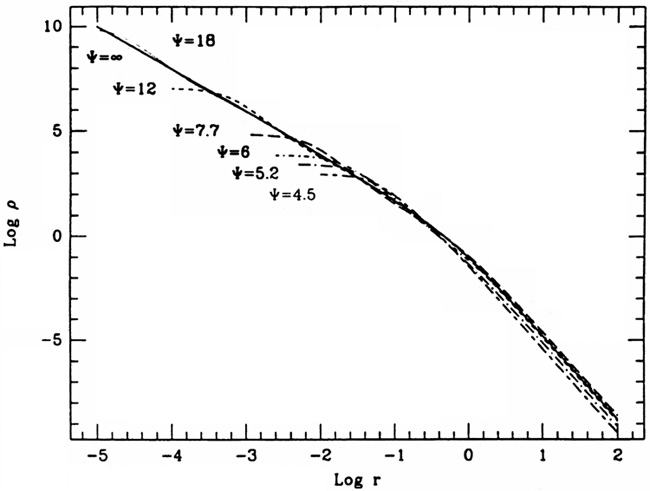Figure 22.10. Behavior of the density profiles for the f models, for different values of the central dimensionless potential (from Bertin, G., Stiavelli, M. 1989, Astrophys. J., 338, 723).

The presence of a concentrated nucleus for high- models induces a rather wide range of exponential behavior ⁽⁵⁶⁾ for the function N(E^*) = d³ xd³ vf (E - E^*) (see Fig. 22.11).

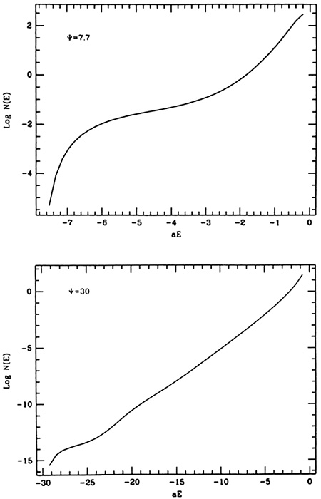Figure 22.11. Behavior of the energy distribution N(E), defined in the text, for two concentrated f models of the sequence (from Bertin, G., Stiavelli, M. 1989, Astrophys. J., 338, 723).

The f models thus constructed provide a surprisingly accurate tool to fit the observations ⁽⁵⁷⁾. In practice they turn out to incorporate the R^1/4 luminosity law, once the relevant photometric profile is obtained from the model by assuming a constant M/L ratio. For the cases where the photometric profile is best known, such as that of NGC 3379 ⁽⁵⁸⁾, an excellent fit is found over a range of eleven magnitudes; for this galaxy the corresponding kinematical profile (i.e., the velocity dispersion projected along the line of sight) is also well fitted out to the outermost available kinematical data point, around R_e (Fig. 22.12). Fits of this kind provide a dynamical measurement of the mass-to-light ratio based on a global modeling. As indicated earlier, the fit is not sensitive to the value of (provided > 7), which may be tuned only in an attempt at fitting also the possibly present small nucleus (but here other problems should be faced; see section 22.2.3). Such generic adequacy of the f models appears to indicate that the global properties of elliptical galaxies are indeed consistent with the scenario of collisionless collapse, which is probably the explanation of the universality of the R^1/4 luminosity profile. The dependence on of the global profiles in the transition range = 4 - 7 might be used to parameterize the departures from the R^1/4 law (i.e. "non-homology") that have sometimes been noted in relatively small ellipticals ⁽⁵⁹⁾.

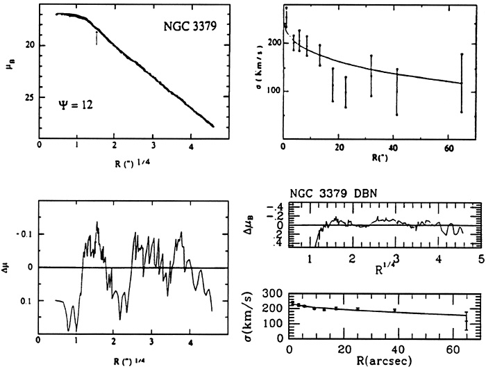Figure 22.12. Photometric and kinematical fit to the galaxy NGC 3379; here µ indicates residual from the best-fit f model (not from R1/4 law). The three larger frames show a fit based on earlier kinematical data, affected by relatively large error bars (from Bertin, G., Saglia, R.P., Stiavelli, M. 1988, Astrophys. J., 330, 78). The remaining part of the figure (bottom right) refers to a fit performed after more accurate kinematical data have become available (from Saglia, R.P., Bertin, G., Stiavelli, M. 1992, Astrophys. J., 384, 433).

This discussion can be extended, at least in part, to non-spherical systems. Some asymptotic analysis can be carried out ⁽⁶⁰⁾ under the ordering () = O(b / c) << 1. At large radii self-consistency leads to an inhomogenous equation for in the variable which can be solved in terms of polynomials (in cos). The analysis shows that concentrated models cannot possess boxy isophotes, while both boxy and disky isophotes may be available at relatively low values of , when a rather wide core is present. Since the asymptotic analysis of the self-consistent non-spherical f models is non-trivial, much insight has been gained by initializing an N-body code with the asymptotic expressions of f with values of b well beyond their expected range of applicability ⁽⁶¹⁾. The simulated systems are found to relax quickly to equilibrium configurations with properties that are not far from those of the approximate equilibrium states (see also Fig. 22.13).

Figure 22.13. A test for the use of spherical f models (from Saglia, R.P., Bertin, G., Stiavelli, M. 1992, Astrophys. J., 384, 433). The F2 model is a highly flattened model (actually, with a dark component included; see following discussion in Sect. 22.3.5) constructed by initializing an N-body simulation with a non-spherical f distribution function with parameters well beyond the allowed limit of quasi-spherical symmetry. The N-body system quickly relaxes to an equilibrium configuration which, from some viewing angle, is as flat as an E4 galaxy (see the ellipticity and position angle of the projected density contours, in the left frames, shown on the radial range out to 4Re). In a simulated observation, this model is looked at from two viewing angles, one where it resembles an E0 galaxy (central frames) and one where it appears as an E4 (right frames). The figure shows the result of a photometric and kinematical fit performed using the analytically simpler spherical (two-component) f models. The results are then used to evaluate the reliability of spherical model fits for flat ellipticals.

22.3.4. Density behavior associated with the R^1/4 law

For a very long time it has been believed that the simplest description of a density profile (r) compatible with the observed luminosity distribution, and thus with the R^1/4 law, would be ~ r^-3. Curiously this belief has persisted ⁽⁶²⁾ well after concrete evidence had accumulated against the r^-3 behavior. To some extent this may have been inspired by the popularity of the so-called modified Hubble profile (see section 22.2.2).

If we assume that the R^1/4 empirical law for the luminosity profile holds exactly from the center out to infinity, under the assumption of spherical symmetry, it is possible to carry out an inversion into a volume density profile (r) that, once projected, gives precisely such a law ⁽⁶³⁾. The numerical solution is tabulated. But there is no physical reason to require that the law holds exactly and at every radius, since the data show systematic deviations ⁽⁶⁴⁾ from the R^1/4 profile and sample up to not more than eleven magnitudes. Thus one should compare models directly with the data and use the R^1/4 law only as a zero order reference case.

It is in this light that one should consider the luminosity profiles associated with the f models, that we have discussed above to be characterized by a density profile with two slopes, r^-2 inside, and r^-4 outside, with a rather sharp transition around r_M. At the time when the self-consistent anisotropic f models were constructed, it was realized independently ⁽⁶⁵⁾ that indeed a simple density distribution compatible with the R^1/4 law is

(22.45)

with associated potential

(22.46)

and circular velocity

(22.47)

Here the half-mass radius is given by r_M = b, since M(r) = Mr / (b + r). For this density profile, the form factor introduced in the previous subsection is exactly q = 0.5. It has been shown that this density distribution is qualitatively similar to that of the singular f models ( = ), but quantitatively different, with relative deviations of 10% in the radial range 10^-5 r_M < r < 10²r_M. Thus, although by itself the above density-potential pair says little on the physical origin of the luminosity profile of elliptical galaxies, it is nonetheless a very handy analytical descriptive tool.

Another simple analytical model for the density distribution is ⁽⁶⁶⁾

(22.48)

with associated potential

(22.49)

and circular velocity

(22.50)

Here the half-mass radius is given by r_M = (1 + 2^1/2)b, since M(r) = Mr² / (b + r)². Variations on the same theme, with more freedom on the relevant exponents, have also been considered, especially with the goal of giving a better parametric description of the properties of the inner structure of galaxy cores and cusps ⁽⁶⁷⁾. These models are generally used with a preference for the r^-4 decline at large radii.

22.3.5. Two-component models (with dark matter)

In spite of their simplicity and limitations, the f models appear to capture much of the structure of elliptical galaxies. Except for the small variations associated with the precise value of for the physically interesting part of the sequence ( > 6) and except for the freedom in the choice of the two dimensional scales, all the phase space properties of the models are fixed. This is a proof of the physical interest of the models, since they are found to be realistic a posteriori, with no parameter tuning. Still, such a rigid structure of the models may be embarassing, for two basic reasons. One point of concern is that, as is well known, the universal photometric structure of elliptical galaxies is curiously accompanied by a variety of kinematical profiles (see Chapter 4). So, the very success of the f models in fitting galaxies such as NGC 3379 automatically implies a failure to fit other ellipticals with flatter velocity dispersion profiles, e.g. NGC 4472. The second reason of concern is that, at this stage, the success of the f models supports a scenario where there is no need for dark matter; we recall that the realistic photometric profile is obtained by converting mass density into luminosity under the assumption of a constant M/L ratio. This would be fine, from a methodological point of view. However, we do have evidence for the presence of massive dark halos around spiral galaxies (see Chapter 20). From the physical point of view it would be hard to believe that ellipticals have no dark matter (see Chapter 24).

From the very beginning it has been clear that the observed variety of kinematical profiles could be ascribed basically to two physical factors: in particular, a relatively flat velocity dispersion profile might result from the presence of a dark halo or from the dominance of tangential orbits ⁽⁶⁸⁾.

Following the approach emphasized in this Chapter (and in general in this book), we may leave aside, as unphysical, the idea of populating stellar orbits in an ad hoc manner in order to produce desired velocity dispersion profiles. In doing so, we are also encouraged by general stability arguments which suggest that significant departures from quasi-Maxwellian distributions of stellar orbits are probably a source of collective modes that go in the direction of removing such peculiarities in phase space, as often shown in the context of plasma physics. An additional important semi-empirical argument also confirms this viewpoint. If the variety of kinematical profiles corresponded to the existence of "arbitrary" distributions of stellar orbits, we would expect to observe some kinematical profiles flatter and others steeper than those predicted by the f models; instead, it appears that the steepest observed profiles are those consistent with the one-component f models, for which the drop in velocity dispersion projected along the line of sight from the central regions to R_e is by less than a factor of 2. Furthermore, it is hard to imagine a physical formation scenario leading to basically non-rotating spheroidal systems and to a strong bias of the pressure tensor in the tangential directions. In fact, the scenario of collisionless collapse leads to a bias, but in the radial direction. Therefore the natural option left is to explore the possibility that the observed variety of kinematical profiles results from a variety of situations associated with the presence of dark halos. In other words, we continue to follow the physical scenario of collisionless collapse and ask what would be the impact of the presence of a diffuse halo in the models.

Note that this attempt goes against one intuitive expectation, i.e. that the impressive accuracy of photometric fits based on one-component f models might be spoiled in the presence of a second component. In particular, the influence of a second component would also appear in the relevant virial constraint for the luminous matter that now becomes

(22.51)

where the W_LD term represents the interaction integral. In the spherically symmetric case the self-interaction term can be written as W_L = - q_L GM²_L / r_L while

(22.52)

so that the no dark matter case corresponds to W_LD = 0, q_L 0.5.

A dark halo, if present, is also likely to follow the scenario of collisionless collapse, even if we imagine it to be made of baryonic matter. The simplest way to proceed is thus to devise a two-component analysis where one component contributes to the light and to the observable velocity dispersion profiles, via a constant mass-to-light ratio, and the other contributes as "dark matter" only to the underlying gravitational field. Encouraged by the success of the f function to characterize a scenario of collisionless collapse, we may describe each component by the same form of distribution function, but with independent sets of parameters:

(22.53)

(22.54)

As usual, these expressions hold for E < 0; the functions are taken to vanish for E > 0. The potential entering in the definition of the energy in these functions is the total gravitational potential, generated by the sum of the two contributions _L + _D. The parameter space here involves four dimensionless quantities. In addition to a concentration parameter (_L), one may set three relative scales, i.e. the mass ratio M_L / M_D, the lengthscale ratio r_L / r_D of the corresponding half-mass radii, and the temperature ratio a_L / a_D. In an extensive survey ⁽⁶⁹⁾, about three thousand models have been computed, covering a wide grid in parameter space [especially in the plane (r_L / r_D, M_L / M_D)], mostly addressing the physically plausible case of diffuse halos (i.e. models with r_L/r_D < 1).

The main result of the survey of two-component models is that, in spite of the variety of kinematical profiles generated, there is a natural "conspiracy" for the concentrated models to support realistic luminosity profiles, consistent with the R^1/4 law. A diffuse dark halo may thus alter significantly the velocity dispersion profile with only minor effects on the density distribution of the luminous component. This comes as a surprise, and adds confidence in the overall physical picture at the basis of this model construction. The concept of "minimum halo" can be developed, by analogy with the maximum disk decomposition for spiral galaxies (see Chapter 20). The detailed quantitative properties of the fully self-consistent two-component global models have been used to study the presence of dark halos around elliptical galaxies ⁽⁷⁰⁾ (see Fig. 22.13 and Fig. 22.14). The resulting luminous-dark matter decomposition leads to different values of M_L/M_D (in some galaxies, on the basis of the available kinematical data, which even in the best cases reach out only to R_e, there is no need to invoke the presence of a dark halo), but to a rather well defined value of M_L / L.

Figure 22.14. Intrinsic properties for the best-fit model of NGC 4472, based on two-component f models: density profiles for the dark (D) and the luminous (L) component, cumulative total mass-to-light ratio, circular velocity profile decomposition, and cumulative mass decomposition (from Saglia, R.P., Bertin, G., Stiavelli, M. 1992, Astrophys. J., 384, 433).

Interesting density priority studies of two-component systems have also been carried out ⁽⁷¹⁾ and may be compared with the results of the above survey of distribution function priority models.

⁴⁸ Bertin, G. Stiavelli, M. (1984), Astron. Astrophys., 137, 26; Stiavelli, M., Bertin, G. (1985), Mon. Not. Roy. Astron. Soc., 217, 735; Bertin, G., Stiavelli, M. (1989), Astrophys. J., 338, 723 Back.

⁴⁹ This was realized from the beginning, but a detailed comparison with the observations was made only in a second stage; see Bertin, G., Saglia, R.P., Stiavelli, M. (1988), Astrophys. J., 330, 78 Back.

⁵⁰ Stiavelli, M., Bertin, G. (1987), Mon. Not. Roy. Astron. Soc., 229, 61 Back.

⁵¹ van Albada, T.S. (1982), Mon. Not. Roy. Astron. Soc., 201, 939 Back.

⁵² Lynden-Bell, D. (1967), Mon. Not. Roy. Astron. Soc., 136, 101; Shu, F.H. (1978), Astrophys. J., 225, 83 Back.

⁵³ Merritt, D., Tremaine, S., Johnstone, D. (1989), Mon. Not. Roy. Astron. Soc., 236, 829 Back.

⁵⁴ Bertin, G., Stiavelli, M. (1989), op.cit. Back.

⁵⁵ See Appendix A of Bertin, G., Pegoraro, F., Rubini, F., Vesperini, E. (1994), Astrophys. J., 434, 94 Back.

⁵⁶ Binney, J.J. (1982), Mon. Not. Roy. Astron. Soc., 200, 951 Back.

⁵⁷ See Bertin, G., Saglia, R.P., Stiavelli, M. (1988), op.cit. Back.

⁵⁸ de Vaucouleurs, G., Capaccioli, M. (1979), Astrophys. J. Suppl., 40, 699 Back.

⁵⁹ See Sersic, J.L. (1968), Astron. J., 73, 892; Ciotti, L. (1991), Astron. Astrophys., 249, 91; Prugniel, P., Simien, F. (1997), Astron. Astrophys., 321, 111 and references therein Back.

⁶⁰ Stiavelli, M., Bertin, G. (1985), op.cit. Back.

⁶¹ See Bertin, G., Stiavelli, M. (1989), op.cit.; Saglia, R.P., Bertin, G., Stiavelli, M. (1992), Astrophys. J., 384, 433 Back.

⁶² See statements on p. 940 and 945 in van Albada, T.S. (1982), op.cit. and Fig. 5 in the article by Binney, J.J. (1982), Mon. Not. Roy. Astron. Soc., 200, 951; Smith, B.F., Miller, R.H. (1986), Astrophys. J., 309, 522; White, S.D.M. (1987), in IAU Symposium 127, ed. T. de Zeeuw, Reidel, Dordrecht, p. 339, especially pp. 345-346; White, S.D.M., Narayan, R. (1987), Mon. Not. Roy. Astron. Soc., 229, 103 Back.

⁶³ Young, P.J. (1976), Astron. J., 81, 807 Back.

⁶⁴ E.g., see van Albada, T.S., (1982), op.cit. Back.

⁶⁵ Jaffe, W. (1983), Mon. Not. Roy. Astron. Soc., 202, 995 Back.

⁶⁶ Hernquist, L. (1990), Astrophys. J., 356, 359 Back.

⁶⁷ See Carollo, C.M. (1993), Ph.D. Thesis, Ludwig-Maximilians University, Munich; Dehnen, W. (1993), Mon. Not. Roy. Astron. Soc., 265, 250; Tremaine, S., Richstone, D.O., Byun, Y-I., Dressler, A. et al. (1994), Astron. J., 107, 634 and following papers Back.

⁶⁸ Illingworth, G.D. (1983), in IAU Symposium 100, ed. E. Athanassoula, Reidel, Dordrecht, p.257; Tonry, J.L. (1983), Astrophys. J., 266, 58 Back.

⁶⁹ Saglia, R.P. (1990), Ph. D. Thesis, Scuola Normale Superiore, Pisa; Bertin, G., Saglia, R.P., Stiavelli, M. (1992), Astrophys. J., 384, 423; see also Bertin, G., Saglia, R.P., Stiavelli, M. 1989), in Third ESO-CERN Symposium, eds. Caffo, M. et al., Kluwer, Reidel, p. 303 Back.

⁷⁰ Saglia, R.P., Bertin, G., Stiavelli, M. (1992), Astrophys. J., 384, 433; Saglia, R.P., Bertin, G., Bertola, F., Danziger, I.J., et al. (1993), Astrophys. J., 403, 567; Bertin, G., Bertola, F., Buson, L.M., Danziger, I.J., et al. (1994), Astron. Astrophys., 292, 381 Back.

⁷¹ Ciotti, L., Pellegrini, S. (1992), Mon. Not. Roy. Astron. Soc., 255, 561; Ciotti, L. (1996), Astrophys. J., 471, 68 Back.