


In this section we will discuss the background of relic photons in the universe, or cosmic microwave background, discovered by Penzias and Wilson at Bell Labs in 1963. The discovery of the CMB was revolutionary, providing concrete evidence for the Big Bang model of cosmology over the Steady State model. More precise measurements of the CMB are providing a wealth of detailed information about the fundamental parameters of the universe.
3.1. Recombination and the formation of the CMB
The basic picture of an expanding, cooling universe leads to a number of startling predictions: the formation of nuclei and the resulting primordial abundances of elements, and the later formation of neutral atoms and the consequent presence of a cosmic background of photons, the cosmic microwave background (CMB) [13, 14]. A rough history of the universe can be given as a time line of increasing time and decreasing temperature [15]:
The epoch at which atoms form, when the universe was at an age of 300,000 years and a temperature of around 3000 K is somewhat oxymoronically referred to as "recombination", despite the fact that electrons and nuclei had never before "combined" into atoms. The physics is simple: at a temperature of greater than about 3000 K, the universe consisted of an ionized plasma of mostly protons, electrons, and photons, which a few helium nuclei and a tiny trace of Lithium. The important characteristic of this plasma is that it was opaque, or more precisely the mean free path of a photon was a great deal smaller than the horizon size of the universe. As the universe cooled and expanded, the plasma "recombined" into neutral atoms, first the helium, then a little later the hydrogen.
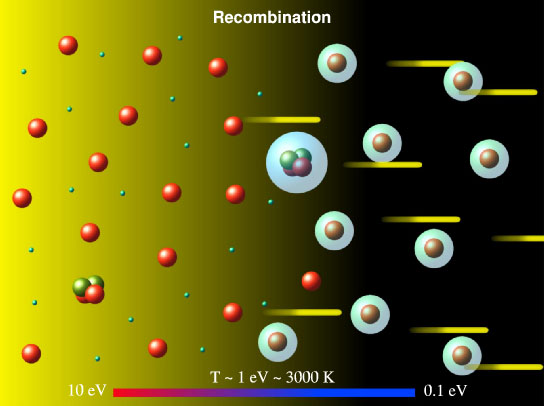 |
Figure 3. Schematic diagram of recombination. |
If we consider hydrogen alone, the process of recombination can be described by the Saha equation for the equilibrium ionization fraction Xe of the hydrogen [16]:
 |
(50) |
Here me is the electron mass and 13.6 eV is the ionization energy of hydrogen. The physically important parameter affecting recombination is the density of protons and electrons compared to photons. This is determined by the baryon asymmetry, or the excess of baryons over antibaryons in the universe. (4) This is described as the ratio of baryons to photons:
 |
(51) |
 b is the
baryon density and h is the Hubble constant in units
of 100 km/s/Mpc,
b is the
baryon density and h is the Hubble constant in units
of 100 km/s/Mpc,
 |
(52) |
Recombination happens quickly (i.e., in much less than a Hubble time
t ~ H-1), but is
not instantaneous. The universe goes from a completely ionized state to
a neutral state over a range of redshifts
 z ~ 200.
If we define recombination as an ionization fraction
Xe = 0.1, we have
that the temperature at recombination TR = 0.3 eV.
z ~ 200.
If we define recombination as an ionization fraction
Xe = 0.1, we have
that the temperature at recombination TR = 0.3 eV.
What happens to the photons after recombination? Once the gas in the
universe is in a neutral state, the mean free path for a photon rises to
much larger than the Hubble distance. The universe is then full of a
background of freely propagating photons with a blackbody distribution
of frequencies. At the time of recombination, the background radiation
has a temperature of
T = TR = 3000 K, and as the
universe expands the photons redshift, so that the temperature of the
photons drops with the increase of the scale factor,
T  a(t)-1. We can detect these
photons today. Looking at the sky, this background of photons comes to
us evenly from all directions, with an observed temperature of
T0
a(t)-1. We can detect these
photons today. Looking at the sky, this background of photons comes to
us evenly from all directions, with an observed temperature of
T0  2.73 K.
This allows us to determine the redshift of the last scattering surface,
2.73 K.
This allows us to determine the redshift of the last scattering surface,
 |
(53) |
This is the cosmic microwave background. Since by looking at higher and higher redshift objects, we are looking further and further back in time, we can view the observation of CMB photons as imaging a uniform "surface of last scattering" at a redshift of 1100.
 |
Figure 4. Cartoon of the last scattering surface. From earth, we see microwaves radiated uniformly from all directions, forming a "sphere" at redshift z = 1100. |
To the extent that recombination happens at the same time and in the same way everywhere, the CMB will be of precisely uniform temperature. In fact the CMB is observed to be of uniform temperature to about 1 part in 10,000! We shall consider the puzzles presented by this curious isotropy of the CMB later.
While the observed CMB is highly isotropic, it is not perfectly so. The largest contribution to the anisotropy of the CMB as seen from earth is simply Doppler shift due to the earth's motion through space. (Put more technically, the motion is the earth's motion relative to a "comoving" cosmological reference frame.) CMB photons are slightly blueshifted in the direction of our motion and slightly redshifted opposite the direction of our motion. This blueshift/redshift shifts the temperature of the CMB so the effect has the characteristic form of a "dipole" temperature anisotropy, shown in Fig. 5.
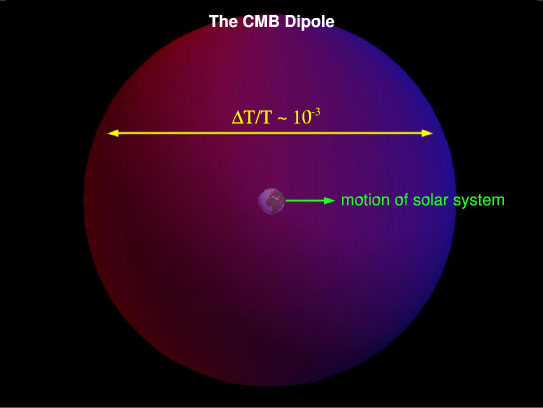 |
Figure 5. The CMB dipole due to the earth's peculiar motion. |
This dipole anisotropy was first observed in the 1970's by
David T. Wilkinson and Brian E. Corey at Princeton, and another group
consisting of George F. Smoot, Marc V. Gorenstein and Richard
A. Muller. They found a dipole variation in the CMB temperature of about
0.003 K, or
(T / T)
10-3,
corresponding to a peculiar velocity of the earth of about
600 km/s, roughly in the direction of the constellation Leo.
The dipole anisotropy, however, is a local phenomenon. Any
intrinsic, or primordial,
anisotropy of the CMB is potentially of much greater cosmological
interest. To describe
the anisotropy of the CMB, we remember that the surface of last
scattering appears to us
as a spherical surface at a redshift of 1100. Therefore the natural
parameters to
use to describe the anisotropy of the CMB sky is as an expansion in
spherical harmonics
Y m:
m:
 |
(54) |
Since there is no preferred direction in the universe, the physics is independent of the index m, and we can define
 |
(55) |
The = 1 contribution is
just the dipole anisotropy,
 |
(56) |
It was not until more than a decade after the discovery of the dipole
anisotropy that the first observation was made of anisotropy for
 2, by the
differential microwave radiometer aboard the Cosmic Background Explorer
(COBE)
satellite [17],
launched in in 1990. COBE observed that the anisotropy at the quadrupole
and higher was two orders
of magnitude smaller than the dipole:
2, by the
differential microwave radiometer aboard the Cosmic Background Explorer
(COBE)
satellite [17],
launched in in 1990. COBE observed that the anisotropy at the quadrupole
and higher was two orders
of magnitude smaller than the dipole:
 |
(57) |
Fig. 6 shows the dipole and higher-order CMB anisotropy as measured by COBE.
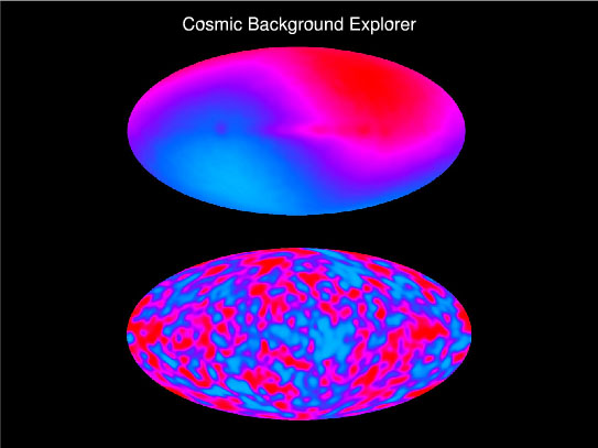 |
Figure 6. The COBE measurement of the CMB
anisotropy
[17].
The top oval is a map of the sky showing the dipole anisotropy
|
It is believed that this anisotropy represents intrinsic fluctuations in the CMB itself, due to the presence of tiny primordial density fluctuations in the cosmological matter present at the time of recombination. These density fluctuations are of great physical interest, first because these are the fluctuations which later collapsed to form all of the structure in the universe, from superclusters to planets to graduate students. Second, we shall see that within the paradigm of inflation, the form of the primordial density fluctuations forms a powerful probe of the physics of the very early universe. The remainder of this section will be concerned with how primordial density fluctuations create fluctuations in the temperature of the CMB. Later on, I will discuss using the CMB as a tool to probe other physics, especially the physics of inflation.
While the physics of recombination in the homogeneous case is quite simple, the presence of inhomogeneities in the universe makes the situation much more complicated. I will describe some of the major effects qualitatively here, and refer the reader to the literature for a more detailed technical explanation of the relevant physics [13]. The complete linear theory of CMB fluctuations was first worked out by Bertschinger and Ma in 1995 [19].
4 If there were no excess of baryons over antibaryons, there would be no protons and electrons to recombine, and the universe would be just a gas of photons and neutrinos! Back.