


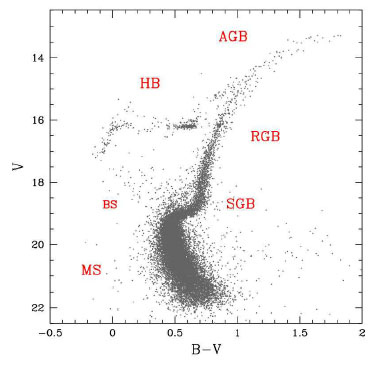
The basic ingredients of a stellar population model are the stellar evolutionary tracks and the stellar model atmospheres. The former trace the evolution of stars of given mass and chemical composition through the various evolutionary phases (Figure 1), providing the basic stellar parameters - bolometric luminosities L; effective temperatures Teff; surface gravities g - as functions of evolutionary timescales. The model atmospheres describe the emergent flux as a function of these parameters, which allows the computation of the stellar spectral energy distribution (SED).
 |
 |
Figure 1. Left-hand panel Observed color magnitude diagram (CMD) of the old, metal-poor galactic GC NGC 1851 (data from [29]). Evolutionary phases are labelled, i.e. Main Sequence (MS); Sub Giant Branch (SGB); Red Giant Branch (RGB); Horizontal Branch (HB); Asymptotic Giant Branch (AGB). BS mean blue stragglers. Right-hand panel. Theoretical H-R diagram of an old, metal-poor SSP, up to the RGB-tip (isochrone from [10]). Solid and dotted linestyles mark Main Sequence and post Main Sequence, respectively. Stellar masses at the turnoff (TO) and RGB-tip are given. |
|
Various sets of stellar tracks exist in the literature, which can be divided into two main groups according to whether the convective overshooting is accounted for or not. Examples of overshooting tracks are the Padova (e.g. [15]), the Geneva ([24]) and the Yale tracks (see Yi, this volume). Stellar tracks which do not include overshooting are those by e.g. [45] and [10]. The actual size of overshooting is still a matter of debate among the various groups, but recent works favour small values (see Yi, this volume). The temperature of the Red Giant Branch is the most discrepant quantity among the stellar tracks, that results in the largest differences among the SSP output. This is shown in Figure 2 that compares the B-V and V-K colors of SSP models with solar metallicity and various ages computed with two different sets of stellar tracks, and the same EPS. While the B-V colors are virtually identical, indicating a consistent modeling of the MS, the V-K colours that depend strongly on the RGB, are very different. A measured V-K ~ 3 is consistent with ages of ~ 5 Gyr or ~ 13 Gyr if the tracks by [37] or by [10] are used, respectively. This agrees with the results by [12], that attribute the large discrepancies in the V-K of their respective models almost entirely to differences in the stellar evolution prescriptions. The temperature of the RGB is determined by the mixing-length parameter, which regulates the stellar radius, hence effective temperatures. In both sets of stellar tracks the mixing-length is calibrated with the solar standard model. The reason of such a discrepancy deserves further investigation.
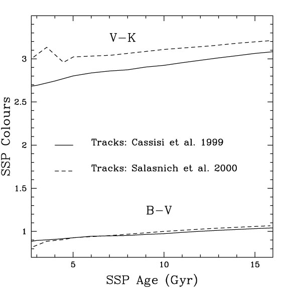 |
Figure 2. Impact of the temperature of the RGB as described by different tracks, on SSP colors. |
The most complete grid of model atmospheres is that by [20] (and revisions), which covers Teff > 3500 K for a wide range of metallicities and gravities, the atmospheres for cooler stars being provided by other groups (e.g. [3]). EPS modellers were forced to make a collage between the various libraries, which could introduce discrepancies in the model results. A recent improvement is due to the works of the Basel group (e.g. [22], [48]), that linked the various available libraries with the Kurucz`s one, and compared the derived temperature-color relations with empirical ones, when available. The resulting library covers virtually the whole parameter space (Teff; g; [Fe/H]) required by theoretical stellar tracks, with the exception of AGB M-type and Carbon stars (see Section 3.6). The spectral resolution of the model atmospheres range between 10 and 20 Å.
Model assumptions are: 1) The stellar initial mass function (IMF),
that provides the mass spectrum of the population. It is common to
express IMFs as declining power-laws with single or multiple slopes,
as it follows from empirical stellar counts. 2) The helium enrichment
law  Y /
Z. 3) The
amount of stellar mass-loss.
Mass-loss is a very critical assumption that impacts on the typical
observables of stellar populations, like colours and
luminosities. Mass-loss occurs in massive stars already on the Main
Sequence. In intermediate mass stars (2 < M /
M
Y /
Z. 3) The
amount of stellar mass-loss.
Mass-loss is a very critical assumption that impacts on the typical
observables of stellar populations, like colours and
luminosities. Mass-loss occurs in massive stars already on the Main
Sequence. In intermediate mass stars (2 < M /
M <
5) it is most
efficient at the Asymptotic Giant Branch (AGB) and determines the fuel
and extension of the Thermally Pulsing AGB phase (herefater
TP-AGB). In low-mass stars mass loss acts already along the Red Giant
Branch (RGB) and determines the morphology of the subsequent
Horizontal Branch (HB) phase. Since the amount of mass loss cannot be
predicted by stellar evolution it must be calibrated with
globular clusters data.
<
5) it is most
efficient at the Asymptotic Giant Branch (AGB) and determines the fuel
and extension of the Thermally Pulsing AGB phase (herefater
TP-AGB). In low-mass stars mass loss acts already along the Red Giant
Branch (RGB) and determines the morphology of the subsequent
Horizontal Branch (HB) phase. Since the amount of mass loss cannot be
predicted by stellar evolution it must be calibrated with
globular clusters data.
The integrated properties of SSP models, e.g. the SED, broad-band
luminosities, magnitudes and colors, are obtained from the integration
of the contributions by individual stars. Two methods in the
literature can be distinguished by the choice of the integration
variable for the stars in the post Main Sequence phase: isochrone
synthesis and fuel consumption-based methods. The right-hand panel of
Figure 1 shows in the theoretical
H-R diagram the isochrone of
a 13 Gyr old metal-poor SSP up to the RGB-tip. The Main Sequence is
populated by stars spanning a large mass range, from ~ 0.1
M to the
turnoff mass. The stellar luminosities are
proportional to a high power of the stellar masses, therefore the
integrated luminosity of the Main Sequence is obtained with an
integration by mass of the stellar luminosities, convolved with the
IMF. In post Main Sequence phases the mass range spanned by living
stars is very small (cf. labels in
Figure 1), and the luminosity is no
longer related primarily to the mass. For the post Main Sequence two
choices are possible. 1) The evolutionary lifetime of one single mass
is adopted as integration variable. In this case the synthesis is
based on the fuel consumption theorem (see
Section 3.3). 2) The
integration by mass is also performed in post-Main Sequence, in which
case the technique is called isochrone synthesis (see
Section 3.4). Pros and cons of the two
methods have been longely discussed in the literature (see e.g.
[11],
[34]).
A recent viewpoint will be given elsewhere.