4. POWER SPECTRUM

The power spectrum (power spectral density) is also a quadratic statistic of the spatial clustering, as is the two-point correlation function. Formally they are equivalent (the power spectrum is the Fourier transform of the correlation function), but they describe different sides of a process. The power spectrum is more intuitive physically, separating processes on different scales. Moreover, the model predictions are made in terms of power spectra. Statistically, the advantage is that the power spectrum amplitudes for different wavenumbers are statistically orthogonal:

(7)

Here (k) is the Fourier amplitude of the overdensity field = ( - ) / at a wavenumber k, is the matter density, a star denotes complex conjugation, E{} denotes expectation values over realizations of the random field, and _D(x) is the three-dimensional Dirac delta function.

If we have a sample (catalog) of galaxies with the coordinates x_j, we can write the estimator for a Fourier amplitude of the overdensity distribution [47] (for a finite set of frequencies k_i) as

where (x) is the position-dependent selection function (the observed mean number density) of the sample and (x) is a weight function that can be selected at will.

The raw estimator for the spectrum is

and its expectation value

where G(k) = |(k)|² is the window function that also depends on the geometry of the sample volume. Symbolically, we can get the estimate of the power spectra by inverting the integral equation

where denotes convolution, P_R is the raw estimate of power, and N is the (constant) shot noise term.

In general, we have to deconvolve the noise-corrected raw power to get the estimate of the power spectrum. A sample of a characteristic spatial size L creates a window function of width of k 1/L, correlating estimates of spectra at that wavenumber interval.

As the cosmological spectra are usually assumed to be isotropic, the standard method to estimate the spectrum involves an additional step of averaging the estimates (k) over a spherical shell k [k_i, k_{i + 1}] of thickness k_{i + 1} - k_i > k = 1/L in wavenumber space.

As the data set get large, straight application of direct methods (especially the error analysis) becomes difficult. There are different recipes that have been developed with the future data sets in mind. A good review of these methods is given in Ref. 48.

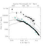
The deeper the galaxy sample, the larger the spectral resolution and the larger the wavenumber interval where the power spectrum can be estimated. Fig. 7 shows the power spectrum for the 2dF survey when contained 160,000 galaxies and had a depth of 750 h^-1 Mpc. The power spectrum was calculated by the 2dF team (filled diamonds) using the direct method [49]. The covariance matrix of this power spectrum estimate was found from simulations of a matching Gaussian Cox process in the sample volume. The diagram shows also the results of the calculation performed by Tegmark et al. [50] over the first public release of the sample containing 102,000 redshifts (squares). Their paper is a good example of application of the large dataset machinery. They used compression of the raw data into (pseudo) Karhunen-Loéve eigenmodes and compressed these quadratically into band-powers, using the Fisher matrix formalism to obtain the final estimate of the power spectrum [1, 48]. For comparison, the power spectrum of the REFLEX cluster sample [51] (obtained by a direct method) is also shown. Clusters of galaxies form only at the highest peaks of the density field. This bias is the responsible for the larger amplitude of the power spectrum corresponding to the clusters of galaxies. The diagram also shows the curves for the power spectrum corresponding to different models of structure formation (see the caption for the details).

Figure 7. The power spectrum of the 2dF galaxy redshift survey calculated using two different estimators [49, 50] and for the X-ray built survey of clusters of galaxies REFLEX (filled circles) [51]. The dashed line correspond to an Einstein-de Sitter (M = 1, = 0) CDM model that is clearly rejected by the observations. The -CDM concordance model (M = 0.3, = 0.7, h = 0.7) is represented by solid lines with the appropriate bias parameters for both galaxies (bottom line) and clusters (top line), (figure from Guzzo [4].)

The main new feature in the spectra, obtained for the new deep samples, is the emergence of details (wiggles). Sometime ago, the goal was to estimate the overall behavior of the spectrum and, at most, to find its maximum, which is related with the homogeneity scale. The new data enables us to see and study the details of the spectrum. These wiggles could be interpreted as traces of acoustic oscillations in the post-recombination power spectrum. Similar oscillations are predicted for the cosmic microwave background radiation fluctuation spectrum. It seems, however, that the apparent wiggles detected in the 2dF power spectrum are an artifact due to the window function and other measurement technicalities [49, 50, 4].